FLIGHT MODEL PHYSICS

This document is a very technical description of the flight model used in Microsoft Flight Simulator. All parameters for it should be defined in the flight_model.cfg file. For documentation on the legacy *.AIR file format, please look at the ESP Flight Models documentation.

 

What is a Flight Dynamics Model?

The problem of simulating a flight can be stated as follows:

 

 

Mathematically speaking, this problem can be expressed under the form of a first-order system of Ordinary Differential Equations of unknown \(\boldsymbol{X}_{\textrm{state}}\):

 

$$\frac{\mathrm{d} \boldsymbol{X}_{\textrm{state}} }{\mathrm{d}t} (t)= H\left(\boldsymbol{X}_{\textrm{state}}(t), \boldsymbol{\delta}_{\textrm{controls}}(t)\right)$$

 

where:

 

\(\boldsymbol{X}_{\textrm{state}}\) is the vector of all primary 6- DoF aircraft state variables which gives, at each time , the exact dynamic configuration of the aircraft:

$$ \begin{array}{lll} \boldsymbol{X}_{\textrm{state}} &= \left( \begin{array}{l} x_G\\ y_G\\ z_G\\ \theta_x\\ \theta_y\\ \theta_z\\ v_{x,G}\\ v_{y,G}\\ v_{z,G}\\ q\\ r\\ p \end{array} \right) & \begin{array}{ll} \left. \begin{array}{l} \\ \\ \\ \end{array} \right\} & \textrm{position}\\ \left. \begin{array}{l} \\ \\ \\ \end{array} \right\} & \textrm{orientation or attitude}\\ \left. \begin{array}{l} \\ \\ \\ \end{array} \right\} & \textrm{translational velocity}\\ \left. \begin{array}{l} \\ \\ \\ \end{array} \right\} & \textrm{rotational velocity} \end{array} \end{array} $$

 

\(\boldsymbol{\delta}_{\textrm{controls}}\) is the input control vector that gives each time the state increment of the aircraft controls (rudder, ailerons, spoilers, elevators, etc...) as entered by user:

 

$$\begin{array}{lll} \boldsymbol{\delta}_{\textrm{controls}} & = \left( \begin{array}{l} \delta_{a} \\ \delta_{e} \\ \delta_{r} \\ \delta_{s}\\ \end{array} \right) & \begin{array}{l} \textrm{ailerons}\\ \textrm{elevators}\\ \textrm{rudder}\\ \textrm{spoilers} \end{array} \end{array}$$

 

\(H\) is a complicated vectorial function - generally non-linear - describing how the aircraft responds to user inputs according to the fundamental equations of solid dynamics (6 DoF):

 

 

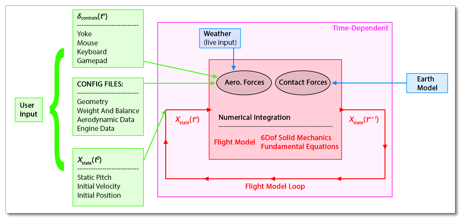
In the following sections we will go into the details of each aspect of this equation, notably what this \(H\) function is exactly, and we will explain how the equation is solved numerically to update the aircraft state.

 

 

Aircraft description - Wing Geometry

The projection of the wing of the plane on the \(x-z\) plane is called the wing planform. A typical planform is sketched below:

 

 

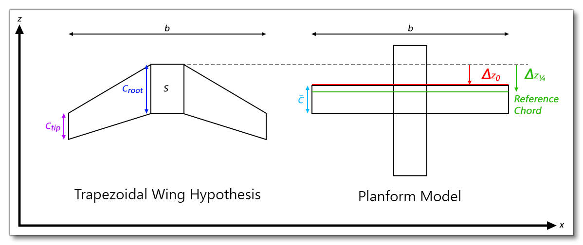
• \(S\) is the total wing area, the area of the planform, where:
  $$S = \int_{-\frac{b}{2}}^{\frac{b}{2}}{c(x)\mathrm{d}x}$$
• \(b\) is the wing span, the maximum lateral extent of the planform
• \(c_{tip}\) is the chord at the tip
• \(c_{root}\) is the chord at the root
• \(\lambda =\frac{c_{tip}}{c_{root}}\) is the tapper ratio
• \(AR=\frac{b^2}{S}\) is the aspect ratio of the planform
• \(\Lambda_n\) is the sweep angle of any constant-chord fraction i.e: the angle formed by \(\boldsymbol{e}_x\) and the line linking all the points located at distance \((1/n)\,c(x)\) from the leading edge. For instance, \(\Lambda_0\) corresponds to the angle between the leading edge and lateral direction \(\boldsymbol{e}_x\).
• \(\Gamma\) is the dihedral angle of the wing

 

A wing section, or airfoil, is simply a cut through of the lifting surface along the plane of a constant \(x\):

 

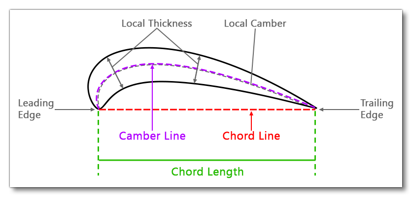
Several quantities are associated with a sectional airfoil:

• \(c=c(x)\) is the local section chord size
• \(\epsilon = \epsilon(x)\) is the section angular twist with respect to the root section
• \(\alpha = \alpha(x)\) is the deviation of the angle of attack for section \(x\) with respect to the angle of attack at wing root section, which is the angle of attack taken as reference for the simulation

From this purely geometric data, we can compute several data sets of major interest in aerodynamics theory:

 

\(\bar{c}\) the MAC of the wing:

$$\bar{c} = \frac{2}{S}\int_{0}^{\frac{b}{2}}{c^2(x)\mathrm{d}x}$$

 

The MAC can be considered a two-dimensional representation of the whole wing. The pressure distribution over the entire wing can be reduced to a single lift force on and a moment around the aerodynamic center of the MAC (that we will define just below). Therefore, not only the length but also the position of MAC is often important. In particular, the position of the CG of an aircraft is usually measured relative to the MAC, as the percentage of the distance from the leading edge of MAC to CG with respect to MAC itself. In the same manner as we have reduced all the chords \(c(x)\) to a single MAC chord \(\bar{c}\), we can reduce all the positions of the points \(z_n(x)\) located at a fraction \(n\) from the leading edge of the local chord \(c(x)\) to a single averaged position \(\bar{z}_n\).

 

\(\Delta \bar{z_{n}} = z_{\textrm{wing apex}} - \bar{z_{n}}\) the longitudinal location of this averaged chord-fraction point on the MAC with respect to wing apex is then:

$$\Delta \bar{z}_{n} = \frac{2}{S}\int_0^{\frac{b}{2}}{\Delta z_n(x)\,c(x)\mathrm{d}x}$$

 

All these quantities can be analytically computed for a trapezoidal tappered swept wing like the one depicted in at the top of this section. In this specific case, we get:

$$S = b\, c_{root}\frac{1+\lambda}{2}$$

The sweep angle of any constant chord fraction line can be related to that of the leading edge sweep angle by:

$$AR\, \textrm{tan}\Lambda_n = AR\, \textrm{tan}\Lambda_0 -4 n \frac{1-\lambda}{1+\lambda}$$

 

The equivalent planform MAC is:

$$\bar{c} = \frac{2\left(1+\lambda+\lambda^2\right)}{3\left(1+\lambda\right)} c_{root}\,$$

 

The location of any chord-fraction \(n\) point on the MAC relative to the wing apex is:

$$\Delta \bar{z}_{n} = \bar{c}\left(n+\frac{(1+\lambda)\,(1+2\lambda)}{8\,(1+\lambda+\lambda^2)}\, \textrm{AR} \, \textrm{tan}\Lambda_0\right) = n \bar{c} + \frac{b}{6}\left(\frac{1+2\lambda}{1+\lambda}\right)\textrm{tan}\Lambda_0$$

 

For instance, the longitudinal position of the leading edge of the equivalent planform - called the reference chord in Microsoft Flight Simulator - in body coordinate system centered at VMO is:

$$z_{\textrm{ref chord}} = z_{\textrm{wing apex}} - \Delta \bar{z}_{0} = z_{\textrm{wing apex}} - \frac{b}{6}\left(\frac{1+2\lambda}{1+\lambda}\right)\textrm{tan}\Lambda_0$$

 

The placing of the MAC leading edge (reference chord) at the correct position along the airplane body is important for a correct CG indication in gauges However, it does not affect flight dynamics. This means that the only wing geometrical parameters influencing the simulation are:

• \(S\)
• \(b\)
• \(c_{root}\)
• wing incidence (the influence on AoA on lift calculation)

From them the math computes as:

• \(c_{tip} = \frac{2S}{b} -c_{root}\)
• \(\lambda = \frac{c_{tip}}{c_{root}}\)
• \(\bar{c} = \frac{2\left(1+\lambda+\lambda^2\right)}{3\left(1+\lambda\right)} c_{root}\,\)
• \(AR = \frac{b^2}{S}\)

 

 

Aircraft Description - Aerodynamics

Below we explain a bit about the physics of the aerodynamics of the flight model.

 

Aerodynamic Coefficients

The lift, drag and pitching moments are dimensional coefficients of the wing which would be defined as:

• Lift coefficient \(C_L = \frac{L}{QS}\)
• Drag coefficient \(C_D = \frac{D}{QS}\)
• Pitching moment coefficient \(C_m = \frac{M}{QS\bar{c}}\), by convention it is generally computed with respect to quarter-chord point of the airfoil (i.e aerodynamic center)

 

Here \(Q = \frac{1}{2}\rho u_z^2\) is the dynamic pressure and \(L\), \(D\) and \(M\) are respectively the lift force, the drag force and the pitching moment.

 

Pressure Center

The pressure center \(P_{pc}(x)\) is the physical point of application of the resulting aerodynamic forces, generally taking into account only the lift force. Its position depends on the way the local pressure forces are located around the airfoil section. It can be evaluated from the pitch moment and the lift. We note \(z_{pc}(x)\) the longitudinal position of \(P_{pc}\) with respect to the longitudinal position of the point \(P\) at which the pitching moment has been evaluated:

$$\frac{z_{pc}(x)}{c(x)} = -\frac{c_{m,P}(x)}{c_{\ell}}(x)$$

 

This point moves depending on the angle of attack. When the angle of attack is zero, it is located about 3/4 of the chord from the leading edge, and moves forward as the angle of attack increases, until it's a maximum of 30% of the chord from the leading edge.

 

Aerodynamic Center

The section aerodynamic center \(P_{ac} = P_{ac}(x)\) of an airfoil is the point about which the pitching moment, due to the distribution of aerodynamic forces acting on the airfoil surface, is independent of the angle of attack.

$$\frac{\mathrm{d} c_{m, P_{ac}} }{\mathrm{d} \alpha}(x) = 0$$

 

Thin-airfoil theory tells us that the aerodynamic center is located on the chord line, one quarter of the way from the leading to the trailing edge - the so-called quarter-chord point. The value of the pitching moment about the aerodynamic center can also be determined from thin-airfoil theory, but requires a detailed calculation for each specific shape of camber line. Here, we simply note that, for a given shape of camber line the pitching moment about the aerodynamic center is proportional to the amplitude of the camber, and generally is negative for conventional subsonic (concave down) camber shapes.

 

We note \(\Delta z_{ac} = z_{P}(x) - z_{ac}\) the longitudinal position of \(P_{ac}\) where \(P\) is the point at which the pitching moment has been evaluated. The moment computed with respect to point \(P_{ac}\), for the section at lateral position:

$$\begin{array}{ll}
&\displaystyle c^2 \, c_{m, P_{ac}}= \left(z_{ac}- z_{pc} \right) \, c \, c_{\ell} \\
\Rightarrow & \displaystyle c_{m, P_{ac}} = \left(z_{ac}- z_{pc} \right) \, \frac{c_{\ell}}{c} = -z_{pc}\frac{c_{\ell}}{c} + z_{ac}\frac{c_{\ell}}{c} = c_{m,P} + \Delta z_{ac}\frac{c_{\ell}}{c}
\end{array}$$

 

To get the position of the aerodynamic center, we derive this expression and equal it to zero, admitting that the position of \(P_{ac}\) is nearly fixed (this is true until the angle of attack remains not too near from stall):

$$\begin{array}{lll}
\displaystyle c_{m, P_{ac}} = c_{m,P} + \Delta z_{ac}\frac{c_{\ell}}{c}&& \\
\displaystyle
\displaystyle \frac{\partial c_{m, P_{ac}} }{\partial \alpha} = 0 & \Rightarrow & \displaystyle \frac{\partial c_{m, P} }{\partial \alpha} + \frac{c_{\ell}}{c} \underbrace{\frac{\partial z_{ac} }{\partial \alpha}}_{\approx 0} + \frac{z_{ac}}{c} \frac{\partial c_{\ell} }{\partial \alpha}= 0\\
&\displaystyle \Rightarrow & \displaystyle \Delta z_{ac} = c \frac{\partial c_{m,P}}{\partial c_{\ell}}
\end{array}$$

 

So far, we have computed the aerodynamic center for an airfoil section. The total wing aerodynamic center is defined considering the planform model of the wing. Similarly, we get:

$$\Delta z_{ac} = \bar{c} \frac{\partial c_{m,P}}{\partial c_{\ell}}$$

 

The longitudinal coordinate of the aerodynamic center is thus:

$$z_{ac} = z_P - \Delta z_{ac}\,$$

 

We see that if \(P\) is the aerodynamic center, i.e: the point at which the pitch moment does not vary with lift/AoA, then the derivative is 0 and \(\Delta z_{ac} = 0\).

 

When \(P\) is located exactly at the aircraft gravity center, \(G\), the formula \(\frac{\partial c_{m,G}}{\partial c_{\ell}} = C_{\textrm{static margin}}\) is called the static margin and the aerodynamic center can be computed in the body coordinates system \((0, 0, z_G - \bar{c} \,C_{\textrm{static margin}})\).

 

For a thin airfoil, it can be seen experimentally that the aerodynamic center is located at 1/4 of the chord from the leading edge, and remains nearly fixed in un-stalled standard flight configurations.

 

By default, in Microsoft Flight Simulator:

• Roll and yaw moments tables ( AoA tables and stability derivatives) are assumed to be computed using VMO as reference point for moment computation. The consequence is that if user only has tables generated using a different reference point, a correction must be applied. Note that no correction is applied in aero forces kinetic moment computation to take into account the fact that the angular moments equation is written with respect to \(G\). Best way to circumvent this inconsistency for now is to set \(VMO = G\).
• Pitching moments tables, the location of the point used to create the tables can be explicitly set in flight_model.cfg file under the form of a longitudinal offset with respect to VMO. If no longitudinal offset is set, it is automatically considered that pitch moment tables are defined relative to the wing aerodynamic center. The kinetic moment correction accounting for the fact the \(c_m\) is relative to \(P_{ac}\) and not \(G\) is accurately computed. The code automatically evaluates the aerodynamic center of the wing \((0, 0, z_G - \bar{c} \,C_{\textrm{static margin}})\), assuming:
  $$\frac{\partial c_{m,G}}{\partial c_{\ell}} \approx \frac{\partial c_{m,ac}}{\partial c_{\ell}}$$

 

Neutral Point

This is the equivalent of the aerodynamic center but taking into account for the lift induced pitch of the whole plane (especially the tail) instead of only taking into account the wing lift.

 

 

Aircraft Mechanical Description

The following details the physics related to aircraft 6 DoF mechanical description.

 

Center Of Gravity

The empty aircraft gravity center position \(\boldsymbol{x}_G^{empty, r}\) is prescribed by the user relative to the Datum Reference Point (in ft in the flight_model.cfg file, using the parameter empty_weight_CG_position.

 

Mass Properties

Let us note \(m_{empty}\) as the mass of the aircraft when it is empty. It is prescribed in lbs using the parameter empty_weight_CG_position in the flight_model.cfg file.

 

It is possible to specify an arbitrary number of additional payload stations (passengers, luggage) in Microsoft Flight Simulator. The maximum number of stations is prescribed in the flight_model.cfg file, using the parameter max_number_of_stations.

 

Each payload is defined by:

• its name
• its weight - \(m_{payload,i} g_{sea level}\)
• its position - \(\boldsymbol{x}_{payload,i}^r\)

 

The position of each payload is given relative to the Datum Reference Point (in ft. Note that if additional payloads are set, Microsoft Flight Simulator will recompute:

• the new total mass - \(m = m_{empty} + \sum_{i}{m_{payload,i}}\)
• the resulting moment of the gravitational forces exerted on these additional payloads
• the new position of the gravity center relative to datum reference
• the new matrix of inertia

 

Aircraft Attitude And Euler Angles

Aircraft orientation is described in terms of Euler angles as illustrated below:

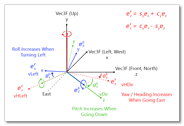
• \(\theta_x\) is the pitch angle
• \(\theta_y\) is the yaw/heading angle
• \(\theta_z\) is the roll/bank angle

Note \(\boldsymbol{\theta} = \left(\theta_x, \, \theta_y, \, \theta_z\right)\) the rotation vector. The 3 rotations corresponding to the 3 Euler angles must be compounded in a given, chosen, arbitrary order to get the global rotation/orientation/attitude of the plane. The is order is yaw - pitch - roll in Microsoft Flight Simulator.

 

Static Longitudinal Stability - Matrix Of Inertia

The matrix of inertia of a solid is symmetric and depends only on the shape and physical nature of the solid object. It is computed relative to a specific point, generally the gravity center \(C_G\):

$$\boldsymbol{\mathcal{J}}_G = \left(
\begin{array}{lll}
\displaystyle \int_{B}{\rho^b \left(\left(y-y_{G}\right)^2+\left(z-z_{G}\right)^2\right)}&
\displaystyle -\int_{B}{\rho^b \left(x-x_{G}\right)\left(y-y_{G}\right)} &
\displaystyle -\int_{B}{\rho^b \left(x-x_{G}\right)\left(z-z_{G}\right)}\\\\
\displaystyle -\int_{B}{\rho^b \left(x-x_{G}\right)\left(y-y_{G}\right)} &\displaystyle \int_{B}{\rho^b \left(\left(x-x_{G}\right)^2+\left(z-z_{G}\right)^2\right)}
&\displaystyle -\int_{B}{\rho^b \left(y-y_{G}\right)\left(z-z_{G}\right)}\\\\
\displaystyle -\int_{B}{\rho^b \left(x-x_{G}\right)\left(z-z_{G}\right)} &\displaystyle -\int_{B}{\rho^b \left(y-y_{G}\right)\left(z-z_{G}\right)} &\displaystyle\int_{B}{\rho^b\left(\left(x-x_{G}\right)^2+\left(y-y_{G}\right)^2\right)}\\
\end{array}
\right)$$

where \(\rho^b\) is the local density of the aircraft body

 

For an aircraft, plane, or helicopter, the expression of the matrix of inertia expressed in the stability frame simplifies due to symmetries in the geometry of the plane - \(J_{xz} = 0\), because when taking any cut parallel to the plane:

• \((Oxz)\), the profil obtained is symmetric relative to axis \(Ox\)
• \((Oxy)\), the profile obtained is symmetric relative to axis \(Oy\)

Only non-diagonal term \(\), \(J_{xy} = 0\) which will be very helpful for solving the fundamental 6- DoF rigid body equations described below.

NOTE: These relations are of course not true anymore if the aircraft is loaded in an asymmetric manner... This case is not fully handled in Microsoft Flight Simulator at the moment

 

 

Referential Frames And Conventions

Five different referential frames are used. They are displayed in the following illustration:

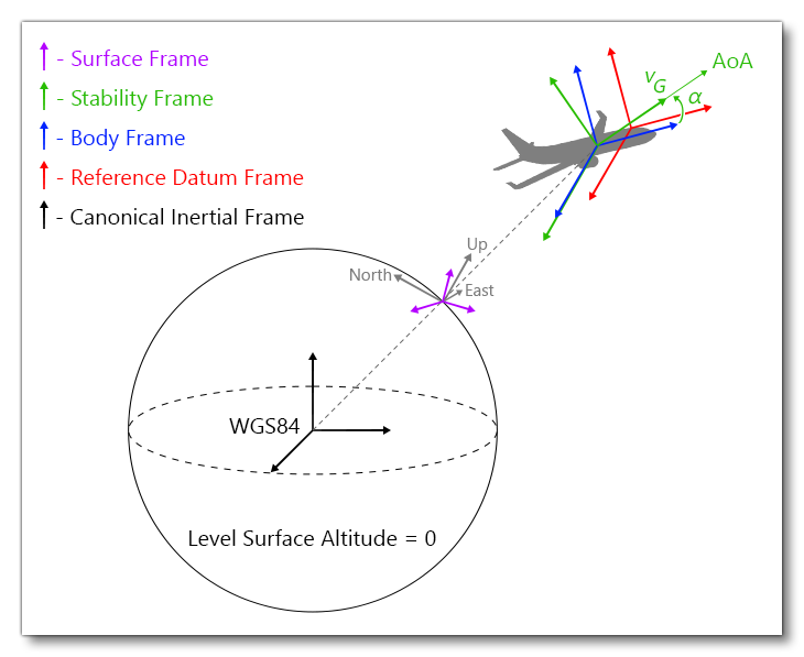
Canonical Inertial Frame

The canonical inertial frame WGS84 is located at the center of the earth and does not move in any way. It is considered as a Galilean frame, on which fundamental laws of solid mechanics can be written. It is the only referential we use which does not move in time.

 

Aircraft Body Frame

This frame \(\left(O_{FSX}(t), \,\boldsymbol{e}_x^b(t), \,\boldsymbol{e}_y^b(t), \,\boldsymbol{e}_z^b(t)\right)\) is attached to the aircraft body. According to historical FSX conventions inherited by Microsoft Flight Simulator it is centered on the centerline chord aft of the leading edge.

 

The \((0,0,0)\) point in the model is the visual center when loaded into Microsoft Flight Simulator. The term "centerline chord" is the ¼ root chord. This is usually the exact same point in the model. By default Microsoft Flight Simulator defines the center of lift as the model's center, which means the center of lift is (by default) defined at the ¼ root chord position.

 

Be careful, this is only true if the modeler did in fact set the model's mesh origin to the ¼ root chord position! If the modeler chose for some reason to set the model's origin at the tip of the aircraft nose, then all bets are off on the model ever being able to be properly configured...

 

Also, be aware that in Microsoft Flight Simulator, this referential is left-handed:

• \(z\) is the longitudinal direction pointing toward the nose of the aircraft; rotation of the aircraft around this axis is named roll or bank
• \(p\) is the roll velocity rate expressed in the body frame
• \(x\) is the side direction pointing toward the right wing typically on a plane; rotation of the aircraft around this axis is named pitch
• \(q\) is the pitch velocity rate expressed in the body frame
• \(y\)is the vertical direction pointing up the aircraft; rotation of the aircraft around this axis is named yaw or heading.
• \(r\) is the yaw velocity rate expressed in the body frame.

 

The body frame is often of interest because the origin and the axes remain fixed relative to the aircraft. This means that the relative orientation of the Earth and body frames describes the aircraft attitude. Also, the direction of the force of thrust is generally fixed in the body frame, though some aircraft can vary this direction, for example by thrust vectoring.

 

To get the transformation matrix from body coordinates to Earth right-handed coordinates, Euler angles are to be compounded in this order: yaw / pitch / roll. Let us adopt the following notation:

$$\begin{array}{lll}
\textrm{yaw}&c_y = \textrm{cos}\,\theta_y,& s_y = \textrm{sin}\,\theta_y\\
\textrm{pitch}&c_x = \textrm{cos}\,\theta_x,& s_x = \textrm{sin}\,\theta_x\\
\textrm{roll}&c_z = \textrm{cos}\,\theta_z,& s_z = \textrm{sin}\,\theta_z
\end{array}$$

 

And let us compound the 3 Euler rotations in the required order yaw / pitch / roll to get the transformation matrix:

$$\begin{array}{lll}
\textrm{yaw}
&
&
\left(
\begin{array}{lll}
\phantom{-}c_y & 0 & -s_y \\
\phantom{-}0 & 1 & 0\\
s_y & 0 & c_y
\end{array}
\right)
\\
\textrm{pitch} &
\left(
\begin{array}{lll}
1 & 0 & 0 \\
0 & \phantom{-}c_x & s_x\\
0 & -s_x & c_x
\end{array}
\right)
&
\left(
\begin{array}{lll}
\phantom{-}c_y & \phantom{-}0 & -s_y \\
s_y s_z& \phantom{-}c_x & s_x c_y\\
c_x s_y & -s_x & c_x c_y
\end{array}
\right)
\\\\
\textrm{roll} &
\left(
\begin{array}{lll}
\phantom{-}c_z& s_z & 0 \\
-s_z & c_z & 0\\
0 & 0 & 1
\end{array}
\right)
&
\left(
\begin{array}{lll}
c_z c_y + s_z s_x s_y & s_z c_x & -c_z s_y + s_z s_x c_y\\
-s_z c_y + c_z s_x s_y & \phantom{-}c_x c_z & s_z s_y +c_z s_x c_y\\
c_x s_y & -s_x & \phantom{-}c_x c_y
\end{array}
\right)
\end{array}$$

 

In the code, the transformation matrix \(\mathcal{R}^{\textrm{body} (z, x, y) \rightarrow \textrm{earth}}\) is given so that vector coordinates in the body frame are given as \((z, x, y)\), which just comes to multiplying the above transformation matrix by the permutation matrix, like this:

$$\begin{array}{lll}
&
\left(
\begin{array}{lll}
c_z c_y + s_z s_x s_y & -s_z c_y + c_z s_x s_y & c_x s_y \\
s_z c_x & \phantom{-}c_x c_z & -s_x\\
-c_z s_y + s_z s_x c_y & s_z s_y +c_z s_x c_y & \phantom{-}c_x c_y
\end{array}
\right)
&
\left.
\left(
\begin{array}{lll}
0& 1 & 0 \\
0 & 0 & 1\\
1 & 0 & 0
\end{array}
\right)
\right\} \left(z, x, y\right) \rightarrow \left(x, y, z\right)
\\\\
\underbrace{
\left(
\begin{array}{lll}
0 & 0 & 1 \\
1 & 0 & 0\\
0 & 1 & 0
\end{array}
\right)
}_{ y \leftrightarrow z \textrm{, earth right-handed} (x, y, z) \rightarrow (z, x, y)}
&
\left(
\begin{array}{lll}
-c_z s_y + s_z s_x c_y & s_z s_y +c_z s_x c_y & \phantom{-}c_x c_y\\
c_z c_y + s_z s_x s_y & -s_z c_y + c_z s_x s_y & c_x s_y\\
s_z c_x & \phantom{-}c_x c_z & -s_x\\
\end{array}
\right)
&
\left(
\begin{array}{lll}
\phantom{-}c_x c_y & -c_z s_y + s_z s_x c_y & s_z s_y +c_z s_x c_y \\
c_x s_y & c_z c_y + s_z s_x s_y & -s_z c_y + c_z s_x s_y \\
-s_x & s_z c_x & \phantom{-}c_x c_z \\
\end{array}
\right)
\end{array}$$

 

We finally get the expression of this transformation matrix as found in the code:

$$\mathcal{R}^{\textrm{body} (z, x, y) \rightarrow \textrm{earth}}
=
\left(
\begin{array}{lll}
c_x c_y & s_z s_x c_y - c_z s_y & c_z s_x c_y + s_z s_y\\
c_x s_y & s_z s_x s_y + c_z c_y & c_z s_x s_y -s_z c_y \\
- s_x & s_z c_x & c_z c_x
\end{array}
\right)$$

 

 

Surface Frame

The equation for the surface reference frame is noted as: \(\left(H(t), \boldsymbol{e}_x^{surf}(t), \boldsymbol{e}_{y}^{surf}(t), \boldsymbol{e}_{z}^{surf}(t)\right)\)

 

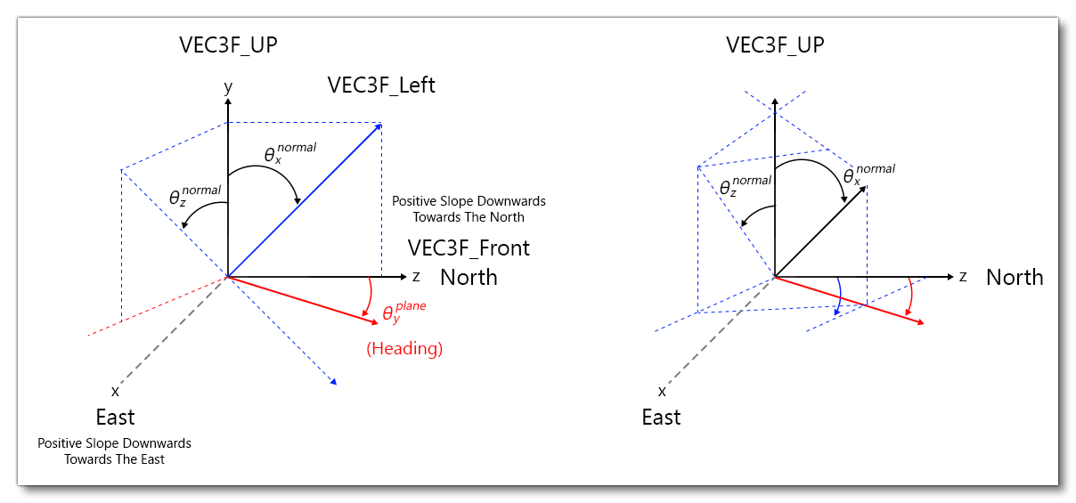
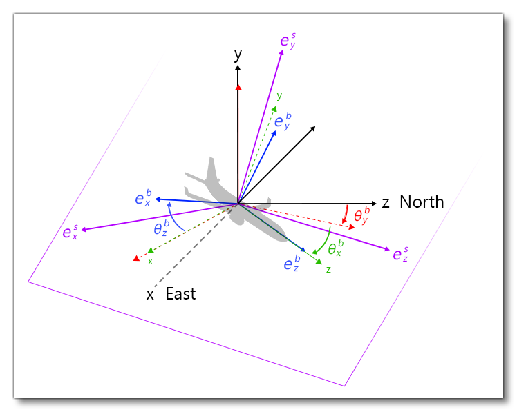
The center of the surface frame is the localization of the current projection \(H(t)\) of the gravity center \(C_G(t)\) of the plane on the geoid model ( AMSL). The surface frame \(\left(H, \boldsymbol{e}_{x}^{s}(t), \boldsymbol{e}_{y}^{s}(t), \boldsymbol{e}_{z}^{s}(t)\right)\) is defined as shown in the following image:

 

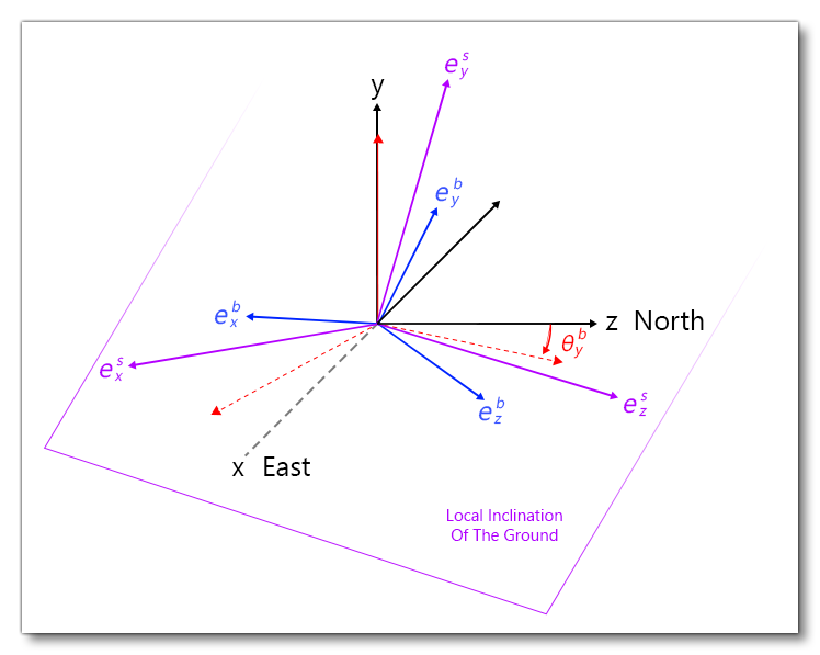
The yaw of this reference frame is equal to the current yaw of the aircraft body frame, the pitch and roll are obtained by analyzing the local surface normal pitch and roll:

$$\theta_x^{nor} = \textrm{atan}{\left(\frac{n_z}{n_y}\right)}\,, \quad \theta_z^{nor} = \textrm{atan}{\left(\frac{n_x}{n_y}\right)}$$

$$\begin{array}{ll}
\boldsymbol{n} &= \displaystyle \left(
\begin{array}{l}
\textrm{cos}\left(\frac{\Pi}{2}-\theta_z^{nor}\right)\,\textrm{sin}\left(\theta_x^{nor}\right)\,\textrm{cos}\left(\theta_y^{nor}\right) + \textrm{sin}\left(\frac{\Pi}{2}-\theta_z^{nor}\right)\,\textrm{sin}\left(\theta_y^{nor}\right)\\
\textrm{cos}\left(\frac{\Pi}{2}-\theta_z^{nor}\right)\,\textrm{sin}\left(\theta_x^{nor}\right)\,\textrm{sin}\left(\theta_y^{nor}\right) - \textrm{sin}\left(\frac{\Pi}{2}-\theta_z^{nor}\right)\,\textrm{cos}\left(\theta_y^{nor}\right) \\
\textrm{cos}\left(\frac{\Pi}{2}-\theta_z^{nor}\right)\,\textrm{cos}\left(\theta_x^{nor}\right)
\end{array}
\right)\\\\
&= \displaystyle \left(
\begin{array}{l}
\textrm{sin}\left(\theta_z^{nor}\right)\,\textrm{sin}\left(\theta_x^{nor}\right)\,\textrm{cos}\left(\theta_y^{nor}\right) + \textrm{cos}\left(\theta_z^{nor}\right)\,\textrm{sin}\left(\theta_y^{nor}\right)\\
\textrm{sin}\left(\theta_z^{nor}\right)\,\textrm{sin}\left(\theta_x^{nor}\right)\,\textrm{sin}\left(\theta_y^{nor}\right) - \textrm{cos}\left(\theta_z^{nor}\right)\,\textrm{cos}\left(\theta_y^{nor}\right) \\
\textrm{sin}\left(\theta_z^{nor}\right)\,\textrm{cos}\left(\theta_x^{nor}\right)
\end{array}
\right)\\\\
&= \displaystyle \left(
\begin{array}{l}
\textrm{sin}\left(\theta_z^{nor}\right)\,\textrm{sin}\left(\theta_x^{nor}\right) \\
- \textrm{cos}\left(\theta_z^{nor}\right) \\
\textrm{sin}\left(\theta_z^{nor}\right)\,\textrm{cos}\left(\theta_x^{nor}\right)
\end{array}
\right)\\\\
& \displaystyle =
\left(
\begin{array}{l}
\textrm{cos}\left(\theta_z^{s}\right)\,\textrm{sin}\left(\theta_x^{s}\right)\,\textrm{cos}\left(\theta_y^{b}\right) + \textrm{sin}\left(\theta_z^{s}\right)\,\textrm{sin}\left(\theta_y^{b}\right)\\
\textrm{cos}\left(\theta_z^{s}\right)\,\textrm{sin}\left(\theta_x^{s}\right)\,\textrm{sin}\left(\theta_y^{b}\right) - \textrm{sin}\left(\theta_z^{s}\right)\,\textrm{cos}\left(\theta_y^{b}\right) \\
\textrm{cos}\left(\theta_z^{s}\right)\,\textrm{cos}\left(\theta_x^{s}\right)
\end{array}
\right)
\end{array}$$

 

We compute a new normal that has the same pitch and roll as the "real" normal but which has the same yaw as the aircraft body.

 

Now we just have to find \(\theta^s_x\) and \(\theta^s_z\) such that:

$$\left\{
\begin{array}{l}
\displaystyle s_z^n s_x^n = c_z^s s_x^s \,\textrm{cos}\theta_y^b + s_z^s\textrm{sin}\,\theta_y^b\\\\
\displaystyle -c_z^n = c_z^s s_x^s \textrm{sin}\,\theta_y^b - s_z^s\textrm{cos}\,\theta_y^b\\\\
\displaystyle s_z^n c_x^n = c_z^s c_x^s
\end{array}
\right.$$

$$\left\{
\begin{array}{ll}
\displaystyle (1)\times\textrm{cos}\theta_y^b + (2) \times \textrm{sin}\,\theta_y^b \Rightarrow & \displaystyle s_z^n s_x^n \textrm{cos}\theta_y^b -c_z^n\textrm{sin}\,\theta_y^b = c_z^s s_x^s \\\\
\displaystyle (1)\times\textrm{sin}\theta_y^b - (2) \times \textrm{cos}\,\theta_y^b \Rightarrow & \displaystyle s_z^n s_x^n \textrm{sin}\,\theta_y^b + c_z^n \textrm{cos}\,\theta_y^b = s_z^s\\
\end{array}
\right.$$

 

Then by combining linearly the different lines:

$$\left\{
\begin{array}{ll}
\displaystyle (1)\times\frac{1}{s_z^n c_x^n = c_z^s c_x^s} \Rightarrow & \displaystyle t_x^n \textrm{cos}\theta_y^b -\frac{c_z^n}{s_z^n c_x^n}\textrm{sin}\,\theta_y^b = t_x^s \\\\
(2)\displaystyle \times\frac{1}{c_z^s = \frac{s_z^nc_x^n}{c_x^s}} = \frac{c_x^s}{s_z^nc_x^n}\Rightarrow & \displaystyle c_x^s t_x^n \textrm{sin}\,\theta_y^b + \frac{c_z^n}{c_z^s} \textrm{cos}\,\theta_y^b = t_z^s\\
\end{array}
\right.$$

 

Which provides values for \(\theta^s_x\) and \(\theta^s_z\).

 

Finally, the transformation matrix from body frame coordinates to surface frame coordinates simply writes like \(\mathcal{R}^{\textrm{body} (z, x, y) \rightarrow \textrm{earth} (z, x, y)}\), using relatives angles and the fact that body and surface frames have the same yaw \(\theta_y^s = \theta_y^b\):

$$\mathcal{R}^{\textrm{body} (z, x, y) \rightarrow \textrm{surf} (z, x, y)}
=
\left(
\begin{array}{lll}
\phantom{-}\textrm{cos}\left(\theta_x^b - \theta_x^s\right) & \textrm{sin}\left(\theta_z^b - \theta_z^s\right) \textrm{sin}\left(\theta_x^b - \theta_x^s\right) & \phantom{-}\textrm{cos}\left(\theta_z^b - \theta_z^s\right) \textrm{sin}\left(\theta_x^b - \theta_x^s\right) \\
\phantom{-}0 & \textrm{cos}\left(\theta_z^b - \theta_z^s\right) & -\textrm{sin}\left(\theta_z^b - \theta_z^s\right) \\
- \textrm{sin}\left(\theta_x^b - \theta_x^s\right)& \textrm{sin}\left(\theta_z^b - \theta_z^s\right) \textrm{cos}\left(\theta_x^b - \theta_x^s\right) & \phantom{-} \textrm{cos}\left(\theta_z^b - \theta_z^s\right) \textrm{cos}\left(\theta_x^b - \theta_x^s\right)
\end{array}
\right)$$

 

Stability Frame (Lift And Drag)

This frame is noted in the equation: \(\left(O_{FSX}(t), \,\boldsymbol{e}_x^{stab}(t), \,\boldsymbol{e}_y^{stab}(t), \,\boldsymbol{e}_z^{stab}(t)\right)\)

 

The current AoA \(\alpha(t)\) of the aircraft is the angle formed between the current longitudinal velocity direction of the aircraft and the current longitudinal direction \(z\) of the body referential:

$$\textrm{tan}\left(\alpha(t)\right)= \frac{v_y^b}{v_z^b}\,, \quad \textrm{sometimes noted } = \frac{w}{u}$$

 

The current side slip angle \(\beta(t)\) of the aircraft is the angle formed between the current side velocity direction of the aircraft and the current longitudinal direction \(z\) of the body referential:

$$\textrm{tan}\left(\beta(t)\right) = \frac{v_x^b}{v_z^b}\,, \quad \textrm{sometimes noted } = \frac{v}{u}$$

 

The stability frame is used for the computation of lift and drag forces. It is just a rotation of the body frame around body frame axis \(\boldsymbol{e}_x^b\) (pitch) of angle \(\alpha = \alpha(t)\) corresponding to the current AoA of the aircraft:

$$\left\{
\begin{array}{ll}
\displaystyle \boldsymbol{e}_x^{\textrm{stab}}(t) &\displaystyle = \boldsymbol{e}_x^b(t)\\
\displaystyle \boldsymbol{e}_y^{\textrm{stab}}(t)& \displaystyle =-\sin{\left(\alpha(t)\right)} \,\boldsymbol{e}_z^b(t) + \cos{\left(\alpha(t)\right)} \,\boldsymbol{e}_y^b(t)\\
\displaystyle \boldsymbol{e}_z^{\textrm{stab}}(t) &\displaystyle = \phantom{-}\cos{\left(\alpha(t)\right)}\, \boldsymbol{e}_z^b(t) + \sin{\left(\alpha(t)\right)} \,\boldsymbol{e}_y^b(t)
\end{array}
\right.$$

 

Reference Datum Frame

This referential \(\left(R_{\textrm{datum}}(t), \,\boldsymbol{e}_x^b(t), \,\boldsymbol{e}_y^b(t), \,\boldsymbol{e}_z^b(t)\right)\) is simply a translation of the body frame from \(O_{FSX}\) to an arbitrary reference datum point \(R\) provided by the aircraft manufacturer or by user for practical purpose. \(R\) coordinates are generally provided in the body frame, i.e: with respect to visual model (mesh) center \(O_{FSX}\). The reference datum point \(R\) is defined by user using reference_datum_position in the [WEIGHT_AND_BALANCE] section of the flight_model.cfg file. The user provides the 3 coordinates \((z, x, y)\) of this point relative to the visual model (mesh) center \(O_{FSX}\) point (long: 1/4 MAC, lat: 0, vert: waterline). Coordinates are provided in ft.

 

It's important to understand that the reference datum position is a value used to define just that. The keyword in any description of "reference datum position" is this: arbitrary. In the real world, all aircraft have a reference datum position. It is typically defined in front of the aircraft's nose at some arbitrary point by the designer. If you leave all values at (0,0,0) in aircraft configuration file, then by default your center of lift, your visual model center and your reference datum position are all in the exact same location. However, if you have the correct reference datum position for the real aircraft and know the offsets of such things as fuel tanks from that reference datum position... then you want to use the reference datum position value in the configuration file to offset it from the (0,0,0) default model center and move it to the real world location. By doing that, you can now use real world measurement information that's based on the real world reference datum to position pretty much anything.

 

The only critical thing to keep in mind is that in Microsoft Flight Simulator, aside from the model's center (0,0,0) which is defined in the model (mesh) file itself, every other positional setting in the aircraft configuration files is relative to the defined reference datum position. Since most modelers don't have access to the "real world engineering data" for the aircraft they are building, they simply set the "reference datum position" to be coincident to the model's center origin, then use educated "guesstimates" to set all the other positional entries... In short, the "reference datum position" is completely optional and arbitrary, and even in the absence of accurate hard engineering data from which to work, it may be set to whatever is most convenient for the modeler.

 

 

Fundamental Equations In Inertial Frame

The Euler equations for solid dynamics are only valid in an inertial frame and read:

$$\left\{
\begin{array}{lll}
\displaystyle m \frac{\mathrm{d}\boldsymbol{v}_G}{\mathrm{d}t} &= ~\sum{\boldsymbol{F}_{ext}} & \displaystyle= \boldsymbol{F}_{\textrm{aero}} + \boldsymbol{F}_{\textrm{engine}} + \boldsymbol{F}_{\textrm{ground reaction}} + \boldsymbol{F}_{\textrm{gravity}} \\\\
\displaystyle \frac{\mathrm{d}\left(\boldsymbol{\mathcal{J}}_G \boldsymbol{\omega}\right)}{\mathrm{d}t} & \displaystyle = ~\boldsymbol{\mathcal{M}}_G\left(\sum{\boldsymbol{F}_{ext}}\right) &= \boldsymbol{\mathcal{M}}_G\left( \boldsymbol{F}_{\textrm{aero}}\right) + \boldsymbol{\mathcal{M}}_G\left(\boldsymbol{F}_{\textrm{engine}}\right) + \boldsymbol{\mathcal{M}}_G\left(\boldsymbol{F}_{\textrm{ground reaction}}\right)\,, \\\\
\displaystyle \textrm{with } & \displaystyle \boldsymbol{\mathcal{M}}_G\left(\boldsymbol{F}\right) & \displaystyle = \int_{B}{ \bigl[\left(\boldsymbol{s}-\boldsymbol{x}_G\right)\wedge \boldsymbol{F} \bigr] }
\end{array}
\right.$$

We have used the fact that the kinetic moment of the gravity forces is zero because these forces are applied at gravity center \(G\) of the object.

 

 

Re-Writing In The Aircraft Body Frame

Things are much more complex in three dimensions than in two dimensions. Indeed, the number of parameters needed to describe the dynamics of a rigid body now equals six, hence the name "6-DoF problem" used for this class of mathematical problems. This means that, contrary to the two-dimensional case, System~() must be fully utilized to compute the movement. Moreover, the directions of \(\boldsymbol{\theta}\) and \(\boldsymbol{\omega}\) are not constant in time anymore, and none of the coefficients of the matrix of inertia remains constant in time when written in the inertial frame. This means that:

$$\frac{\mathrm{d}\left(\boldsymbol{\mathcal{J}}_G\boldsymbol{\omega}\right)}{\mathrm{d}t} ~\neq~ \boldsymbol{\mathcal{J}}_G\frac{\mathrm{d}\boldsymbol{\omega}}{\mathrm{d}t}\,$$

 

as \(\boldsymbol{\mathcal{J}}_G\), written in the canonical basis, is not constant in time anymore.

 

To solve these difficulties, the idea is to rewrite these fundamental relations in aircraft body frame. In this frame, the matrix of inertia is constant in time and, as seen above, it is also simplified as: \(J_{xz} = J_{xy} =0\)

 

In the sequel, we note \(\boldsymbol{\mathcal{R}} = \boldsymbol{\mathcal{R}}(t)\) the matrix enabling to pass from the description in basis \((\boldsymbol{e}^b_{x},\, \boldsymbol{e}^b_{y},\, \boldsymbol{e}^b_{z})\) to the description in fixed canonical basis \((\boldsymbol{e}_{x},\, \boldsymbol{e}_{y},\, \boldsymbol{e}_{z})\):

$$\begin{array}{ll}
\boldsymbol{e}_{x}^b(t) &= r_{1x}(t)\boldsymbol{e}_{x}+ r_{1y}(t)\boldsymbol{e}_{y}+r_{1z}(t)\boldsymbol{e}_{z}\\
\boldsymbol{e}_{y}^b(t) &= r_{2x}(t)\boldsymbol{e}_{x}+ r_{2y}(t)\boldsymbol{e}_{y}+r_{2z}(t)\boldsymbol{e}_{z}\\
\boldsymbol{e}_{z}^b(t) &= r_{3x}(t)\boldsymbol{e}_{x}+ r_{3y}(t)\boldsymbol{e}_{y}+r_{3z}(t)\boldsymbol{e}_{z}
\end{array}$$

$$\boldsymbol{\mathcal{R}} = \boldsymbol{\mathcal{R}}(t) =
\left(
\begin{array}{lll}
r_{1x}(t)&r_{2x}(t)&r_{3x}(t)\\
r_{1y}(t)&r_{2y}(t)&r_{3y}(t)\\
r_{1z}(t)&r_{2z}(t)&r_{3z}(t)
\end{array}
\right)$$

$$\left(
\begin{array}{l}
\boldsymbol{e}_{x}^b(t)\\
\boldsymbol{e}_{y}^b(t)\\
\boldsymbol{e}_{z}^b(t)
\end{array}
\right)
=
\boldsymbol{\mathcal{R}}(t)
*
\left(
\begin{array}{l}
\boldsymbol{e}_{x}\\
\boldsymbol{e}_{y}\\
\boldsymbol{e}_{z}
\end{array}
\right)$$

 

As the two basis are orthonormal, the rotation matrix \(\boldsymbol{\mathcal{R}}(t)\) is always a unitary matrix, i.e: \(\boldsymbol{\mathcal{R}}(t)\boldsymbol{\mathcal{R}}(t)^{T} = \boldsymbol{\mathcal{I}}_3, \, \, \forall\, \, t\), where \(\mathcal{I}_3\) is the identity matrix.

 

Derivation Of Vectors Written In The Body Frame

An arbitrary vector \(\boldsymbol{v}^{b}(t)\) described in aircraft body frame \((\boldsymbol{e}_{x}^b(t),\,\boldsymbol{e}_{y}^b(t),\, \boldsymbol{e}_{z}^b(t))\) has a description \(\boldsymbol{v}(t)\) in the fixed inertial frame. The link between these two representations is given by relation:

$$\boldsymbol{v}(t) ~=~ \boldsymbol{\mathcal{R}}(t)\,\boldsymbol{v}^{b}(t)\,$$

As transformation \(\boldsymbol{\mathcal{R}}(t)\) itself is time dependent, in general:

$$\frac{\mathrm{d}\boldsymbol{v}(t)}{\mathrm{d}t} \ne \boldsymbol{\mathcal{R}}(t)\frac{\mathrm{d}\boldsymbol{v}^{b}(t)}{\mathrm{d}t}\,$$

 

The movement of the aircraft body frame must be taken into account while deriving:

$$\displaystyle \frac{\mathrm{d}\boldsymbol{v}(t)}{\mathrm{d}t} ~=~ \displaystyle \frac{\mathrm{d}\boldsymbol{\mathcal{R}}(t)}{\mathrm{d}t}\boldsymbol{v}^{b}(t)+\boldsymbol{\mathcal{R}}(t)\frac{\mathrm{d}\boldsymbol{v}^{b}(t)}{\mathrm{d}t} ~=~ \frac{\mathrm{d}\boldsymbol{\mathcal{R}}(t)}{\mathrm{d}t}\boldsymbol{\mathcal{R}}^{T}\boldsymbol{v}(t)+\boldsymbol{\mathcal{R}}(t)\frac{\mathrm{d}\boldsymbol{v}^{b}(t)}{\mathrm{d}t}~=~ \displaystyle \boldsymbol{\omega(t)}\wedge {\boldsymbol{v}(t)} + \boldsymbol{\mathcal{R}}(t)\frac{\mathrm{d}\boldsymbol{v}^{b}(t)}{\mathrm{d}t}\,.$$

 

Indeed, by deriving relation \(\boldsymbol{\mathcal{R}}^T(t)\boldsymbol{\mathcal{R}}(t)~=~\boldsymbol{\mathcal{I}}_3\), we get:

$$\begin{array}{ll}
&\displaystyle \frac{\mathrm{d} \boldsymbol{\mathcal{R}}(t)}{\mathrm{d}t} \boldsymbol{\mathcal{R}}^{T}(t)~+~\boldsymbol{\mathcal{R}}(t)\frac{\mathrm{d} \boldsymbol{\mathcal{R}}^T(t)}{\mathrm{d} t}~=~ 0 \\\\
\displaystyle \Rightarrow & \displaystyle\frac{ \mathrm{d} \boldsymbol{\mathcal{R}}}{\mathrm{d} t}(t)\boldsymbol{\mathcal{R}}^{T}(t) ~=~ -\left(\frac{\mathrm{d}\boldsymbol{\mathcal{R}}{\mathrm{d}t}(t)\boldsymbol{\mathcal{R}}}(t)^T\right)^T \textrm{ ( i.e } \frac{\mathrm{d}\boldsymbol{\mathcal{R}}}{\mathrm{d}t}(t)\boldsymbol{\mathcal{R}}(t)^T \textrm{ is skew-symmetric) }\\\\
\displaystyle \Rightarrow & \displaystyle \exists\,\, \boldsymbol{\omega} ~=~ \boldsymbol{\omega}(t) \in\, \mathbb{R}^3, \,\, \frac{\mathrm{d}\boldsymbol{\mathcal{R}}}{\mathrm{d}t}(t)\boldsymbol{\mathcal{R}}^{T}(t) ~=~ \displaystyle \left(
\begin{array}{lll}
\phantom{-}0 & - \omega^b_z(t) & \phantom{-}\omega^b_y(t)\\
\phantom{-}\omega^b_z(t) & \phantom{-}0 & - \omega^b_x(t) \\
- \omega^b_y(t) & \phantom{-}\omega^b_x(t) & \phantom{-} 0
\end{array}
\right) ~=~ \boldsymbol{\omega}(t) \wedge {\cdot}\,,
\end{array}$$

 

with:

$$\boldsymbol{\omega}^b(t) = \left(\omega_x^b(t),\, \omega^b_y(t),\, \omega^b_z(t)\right) = \left(q,\, r, \,p\right)\,$$

 

\(p\) is the roll (bank), \(q\) the pitch and \(r\) the yaw (heading), all these quantities being expressed in the body frame. The first term \( \boldsymbol{\omega}(t)^b \wedge \cdot\) accounts for the movement of the body frame (its rotation) as compared to the inertial frame. \(\boldsymbol{\omega}(t)\) is the instantaneous angular speed of the body frame as compared to the inertial frame, written in the canonical, fixed basis \((\boldsymbol{e}_{x}, \boldsymbol{e}_{y}, \boldsymbol{e}_{z})\). We note \(\boldsymbol{\omega}^b\) this same angular speed written in moving basis \((\boldsymbol{e}^b_{x}(t), \,\boldsymbol{e}^b_{y}(t),\, \boldsymbol{e}^b_{z}(t))\) attached to the body. We have \(\boldsymbol{\omega}(t)=\boldsymbol{\mathcal{R}}(t)\boldsymbol{\omega}^b(t)\). Then, using the invariance property of the cross-product, we have, for any arbitrary vector \(\boldsymbol{v}\):

$$\displaystyle \frac{\mathrm{d}\boldsymbol{v}}{\mathrm{d}t}(t) = \left(\boldsymbol{\mathcal{R}}(t)\boldsymbol{\omega}^b(t)\right)\wedge \boldsymbol{v} + \boldsymbol{\mathcal{R}}(t)\frac{\mathrm{d}\boldsymbol{v}^{b}(t)}{\mathrm{d}t} = \boldsymbol{\mathcal{R}}(t)\left(\boldsymbol{\omega}^b(t)\wedge {\boldsymbol{v}^b(t)} + \frac{\mathrm{d}\boldsymbol{v}^{b}(t)}{\mathrm{d}t}\right)\,$$

 

 

Final Formulation As Used In Microsoft Flight Simulator

The final mathematical formulas using the sim are listed in the sections below.

 

Momentum Conservation Equation

Using Formula~() to rewrite \(\frac{\mathrm{d}\left(\boldsymbol{\mathcal{J}}_G \boldsymbol{\omega}\right)}{\mathrm{d}t}\) in System~(), we get:

$$\begin{array}{lll}
&\displaystyle \frac{\mathrm{d}\left(\mathcal{J}_G\boldsymbol{\omega}\right)}{\mathrm{d}t} ~=~ \boldsymbol{\mathcal{M}}_{G}\left(\sum{\boldsymbol{F}_{ext}}\right) ~\Rightarrow ~ \boldsymbol{\mathcal{R}}(t)\left( {\boldsymbol{\omega}^b}\wedge {\mathcal{J}_G^b\boldsymbol{\omega}^b} ~+~ \frac{\mathrm{d}\left(\mathcal{J}_G^b\boldsymbol{\omega}^b\right) }{\mathrm{d}t}\right) \displaystyle ~=~ \boldsymbol{\mathcal{R}}(t) \boldsymbol{\mathcal{M}}^b_{G}\left(\sum{\boldsymbol{F}_{ext}}^b\right) \\\\
\Rightarrow &\displaystyle {\boldsymbol{\omega}^b}\wedge {\mathcal{J}_G^b\boldsymbol{\omega}^b} ~+~ \frac{\mathrm{d}\left(\mathcal{J}_G^b \boldsymbol{\omega}^b\right) }{\mathrm{d}t} ~=~ \boldsymbol{\mathcal{M}}^b_{G}\left(\sum{\boldsymbol{F}_{ext}}^b\right) ~ \Rightarrow ~ {\boldsymbol{\omega}^b} \wedge {\mathcal{J}_G^b\boldsymbol{\omega}^b} ~+~ \mathcal{J}_G^b\frac{\mathrm{d} \boldsymbol{\omega}^b }{\mathrm{d}t} ~=~ \boldsymbol{\mathcal{M}}^b_{G}\left(\sum{\boldsymbol{F}_{ext}}^b\right)\,,
\end{array}$$

 

and \(\mathcal{J}_G^b\) written in the body referential frame associated with the plane is invariant in time and has helpfully some terms which are zero. Term \({\boldsymbol{\omega}^b}\wedge {\boldsymbol{\mathcal{J}}_G^b\boldsymbol{\omega}^b}\) can be developed as:

$$\left(
\begin{array}{lll}
\phantom{-}0 & - \omega^b_z & \phantom{-}\omega^b_y\\
\phantom{-}\omega^b_z & \phantom{-}0 & - \omega^b_x \\
- \omega^b_y & \phantom{-}\omega^b_x & \phantom{-} 0
\end{array}
\right)
\left(
\begin{array}{lll}
J^b_{xx} & 0 & 0\\
0 & \phantom{-}J^b_{yy} & -J^b_{yz}\\
0 & -J^b_{yz} & \phantom{-}J^b_{zz}
\end{array}
\right)
\left(
\begin{array}{l}
\omega^b_x\\
\omega^b_y\\
\omega^b_z
\end{array}
\right)
\\
=
\left(
\begin{array}{lll}
\phantom{-}0 & - p & \phantom{-}r\\
\phantom{-}p & \phantom{-}0 & - q \\
- r & \phantom{-}q & \phantom{-} 0
\end{array}
\right)
\left(
\begin{array}{lll}
J^b_{xx} & 0 & 0\\
0 & \phantom{-}J^b_{yy} & -J^b_{yz}\\
0 & - J^b_{yz} & \phantom{-}J^b_{zz}
\end{array}
\right)
\left(
\begin{array}{l}
q\\
r\\
p
\end{array}
\right)
\\
=
\left(
\begin{array}{lll}
0 & -pJ^b_{yy}-rJ^b_{yz} & pJ^b_{yz} + rJ^b_{zz}\\
pJ^b_{xx} & qJ^b_{yz}& -qJ^b_{zz}\\
-r J^b_{xx} &qJ^b_{yy} & -qJ^b_{yz}
\end{array}
\right)
\left(
\begin{array}{l}
q\\
r\\
p
\end{array}
\right)
=
\left(
\begin{array}{l}
r \, p\,\left( J^b_{zz} - J^b_{yy}\right)+ J_{yz}\left(p^2-r^2\right)\\
p\,q\,\left(J^b_{xx}-J^b_{zz}\right)+q\,r\,J_{yz}\\
q \, r\,\left( J^b_{yy} - J^b_{xx}\right)- q\,p\,J_{yz}\\
\end{array}
\right)\,$$

 

Which finally leads to the following system of equations for the dynamics of rigid bodies:

$$\begin{array}{ll}
&\displaystyle
\left(
\begin{array}{lll}
J^b_{xx} & 0 & 0\\
0 & J^b_{yy} &-J^b_{yz}\\
0 & -J^b_{yz} & J^b_{zz}
\end{array}
\right)
\left(
\begin{array}{l}
\displaystyle \dot{q}\\
\displaystyle \dot{r}\\
\displaystyle \dot{p}
\end{array}
\right)
+
\left(
\begin{array}{l}
r \, p\,\left( J^b_{zz} - J^b_{yy}\right)+ J_{yz}\left(p^2-r^2\right)\\
p\,q\,\left(J^b_{xx}-J^b_{zz}\right)+q\,r\,J_{yz}\\
q \, r\,\left( J^b_{yy} - J^b_{xx}\right)- q\,p\,J_{yz}\\
\end{array}
\right) = \boldsymbol{\mathcal{M}}^b_{G}\left(\sum{\boldsymbol{F}_{ext}}^b\right) \\\\
\displaystyle
\Leftrightarrow &
\left(
\begin{array}{l}
\displaystyle J^b_{xx}\dot{q} + r \, p\,\left( J^b_{zz} - J^b_{yy}\right)+\left(p^2-r^2\right)\,J_{yz}\\
\displaystyle J^b_{yy}\dot{r}-J^b_{yz}\dot{p} + p\,q\,\left(J^b_{xx}-J^b_{zz}\right)+q\,r\,J_{yz} \\
-J^b_{yz}\dot{r} + J^b_{zz} \dot{p} + q \, r\,\left( J^b_{yy} - J^b_{xx}\right)- q\,p\,J_{yz}
\end{array}
\right)
= \left(
\begin{array}{l}
\displaystyle M^b_{G,x}\\
\displaystyle M^b_{G,y}\\
\displaystyle M^b_{G,z}
\end{array}
\right)
= \left(
\begin{array}{l}
\displaystyle M\\
\displaystyle N\\
\displaystyle L
\end{array}
\right)
\end{array}$$

 

Thanks to the simple form of the matrix of inertia of the aircraft written in the body frame, the pitch momentum equation is de-correlated from the others. This is one of the bonuses we get from having struggled to express these equations in the body frame. We directly get, \(J_{yz} \leftarrow -J_{yz}\).

$$\displaystyle
\Leftrightarrow
\left\{
\begin{array}{ll}
\displaystyle \dot{q}&=\displaystyle \frac{ r \, p\,\left( J^b_{yy} - J^b_{zz}\right)+\left(p^2-r^2\right)\,J_{yz} + M}{J^b_{xx}}\\\\
\displaystyle \dot{r} &=\displaystyle \frac{ \left(q\,r - \dot{p}\right)\,J_{yz} + p\,q\,\left(J^b_{zz}-J^b_{xx}\right) + N}{J^b_{yy}}\\\\
\displaystyle \dot{p}&=\displaystyle \frac{ - \left(q\,p+\dot{r}\right)\,J_{yz} + q \, r\,\left( J^b_{xx} - J^b_{yy}\right)+L}{J^b_{zz}}
\end{array}
\right.\,$$

 

With \(\boldsymbol{\mathcal{M}}^b_{G}\left(\sum{\boldsymbol{F}_{ext}}^b\right)\) given by:

$$\displaystyle \boldsymbol{\mathcal{M}}^b_{G}\left(\sum{\boldsymbol{F}_{ext}}^b\right) = \boldsymbol{\mathcal{R}}(t)^T\boldsymbol{\mathcal{M}}_{G}\left(\sum{\boldsymbol{F}_{ext}}\right)
= = \boldsymbol{\mathcal{R}}(t)^T\left(\boldsymbol{\mathcal{M}}_{G}\left(\boldsymbol{f}_{\textrm{aero}}\right) + \boldsymbol{\mathcal{M}}_{G}\left(\boldsymbol{f}_{\textrm{engine}}\right) + \boldsymbol{\mathcal{M}}_{G}\left(\boldsymbol{f}_{\textrm{ground reaction}}\right)\right)\,$$

 

Quantity Of Movement Conservation Equation

In Microsoft Flight Simulator, for practical reasons, as we have already computed all forces in the aircraft/body referential, we also solve the linear acceleration equation in the body referential frame:

$$\displaystyle m \frac{\mathrm{d}^2\boldsymbol{x}_G^b}{\mathrm{d}t^2} + {\boldsymbol{\omega}^b}\wedge {\boldsymbol{v}_G^b} = \boldsymbol{F}^b_{\textrm{aero}} + \boldsymbol{F}^b_{\textrm{engine}} + \boldsymbol{F}^b_{\textrm{ground reaction}} + \boldsymbol{F}^b_{\textrm{gravity}}\,$$

 

With \(\boldsymbol{\omega}^b = \left(q, \, r, \, p\right)\) and \(\boldsymbol{v}^b_G = \left(v^b_{x, G}, \, v^b_{y, G}, \, v^b_{z, G}\right)\), this leads to:

$$\displaystyle
\Leftrightarrow
\left\{
\begin{array}{ll}
\displaystyle m \,\,\left(\dot{v}_{x, G}^b + r\,{v^b_{z, G}}-p\,{v^b_{y, G}}\right)& \displaystyle = X + {F}^b_{x, \textrm{gravity}}\\\\
\displaystyle m\, \,\left(\dot{v}_{y, G}^b+ p\,{v^b_{x, G}}-q\,{v^b_{z, G}} \right)& \displaystyle = Y + {F}^b_{y, \textrm{gravity}}\\\\
\displaystyle m \,\,\left(\dot{v}_{z, G}^b + q\,{v^b_{y, G}}-r\,{v^b_{x, G}} \right)& \displaystyle = Z + {F}^b_{z, \textrm{gravity}}
\displaystyle
\end{array}
\right.$$

 

It is important to note that the point at which the fundamental equations are written is \(G\), which is different from the center \(O_{FSX}\) of the body aircraft frame which serves as a reference to define coordinates.

 

As the pitching moment coefficient is given relative to the wing aerodynamic center, we have to be careful to transform the aero forces moment to take into account the fact that we must at end express all moments relative to \(G\) for consistency:

$$\boldsymbol{M}_{O}(\boldsymbol{F})= \boldsymbol{OM} \wedge \boldsymbol{F} = \boldsymbol{OG} \wedge \boldsymbol{F} + \boldsymbol{GM} \wedge \boldsymbol{F} = \boldsymbol{OG} \wedge \boldsymbol{F} + \boldsymbol{M}_{G}(\boldsymbol{F})$$

To get \(\boldsymbol{M}_{G}(\boldsymbol{F}_{aero})\), we just have to correct the moment \(\boldsymbol{M}_{O}(\boldsymbol{F}_{aero})\) we computed with aerodynamic coefficients with this term \(-\boldsymbol{OG} \wedge \boldsymbol{F}_{aero}\) and \(\boldsymbol{OG}\) is given by the simulation code.

 

For roll moment, this correction is not applied as it is assumed that \(G\) and \(O\) are located on the centerline \(x_O=x_G\) and \(y_O=y_G\).

 

 

Numerical Integration At Each Time Step

This section outlines how some variables are handles each time step of the simulation.

 

Primary Variables

• Body center position (can be transformed in longitude, latitude and altitude): \(\boldsymbol{x}_G = \left(x^n_G,\, y^n_G, \,z^n_G\right)\)
• Body center velocity: \(\boldsymbol{v}_G = \left(v_{x,G}^n,\, v_{y,G}^n, \,v_{z,G}^n\right)\)
• Body orientation (rotation): \(\boldsymbol{\theta} = \left(\theta^n_x, \,\theta^n_y, \,\theta^n_z\right)\)
• Body rotation velocity: \(\boldsymbol{\theta} = \left(q^n = \omega_x^n, \,r^n = \omega_y^n, \,p^n = \omega_z^n\right)\)

Environment Variables

Mostly from altitude and atmosphere model:

• Air density \(\rho\)
• Speed of sound \(c\)
• Ambient wind

 

Secondary Variables

• Relative air speed in body axis
• Total relative speed \(U\)
• Mach number \(M_a = \frac{U}{c}\)
• Dynamic pressure \(Q = \frac{1}{2} \rho U^2\)
• Angle of attack \(\alpha\)
• \(\mathcal{R}^n_{\textrm{stab} \rightarrow \textrm{body}}\)

 

$$\mathcal{R}^n_{\textrm{stab} \rightarrow \textrm{body}} =
\left(
\begin{array}{lll}
1 & 0 & 0\\
0 & \textrm{cos}(\alpha) & -\textrm{sin}(\alpha)\\
0 & \textrm{sin}(\alpha) & \phantom{-}\textrm{cos}(\alpha)
\end{array}
\right)$$

Drag force in classical aerodynamics is positive when pointing toward the back of the plane. Thus a -1 factor must be applied to the \(z\) column of the \(\mathcal{R}^n_{\textrm{stab} \rightarrow \textrm{body}}\) transformation to take into account that in Microsoft Flight Simulator, \(z\) points forward (left-handedness)

• Angle of side slip \(\beta\)
• Rotational velocity in stability frame: pitch velocity in stability frame, roll (bank) velocity in stability frame, yaw (heading) velocity in stability frame:
  $$\left[ \mathcal{R}^n_{\textrm{stab} \rightarrow \textrm{body}}\right]^{-1} \left(
  \begin{array}{l}
  q\\r\\p
  \end{array}
  \right)
  = $$
• \(\dot{\alpha}\)

 

 

Handling Time Step

The numerical integration is the computation that enables to compute unknown quantities at \(t^{n+1}\) from already computed quantities. In Microsoft Flight Simulator, we only use quantities at \(t^n\) and \(t^{n-1}\) and do not go further back in time. The integration method used in Microsoft Flight Simulator is a trapezoidal integration, i.e for a model equation of unknown \(u\) like:

$$\frac{\textrm{d} u}{\textrm{d} t} = F(u, t)$$

 

The value of \(u\) at time \(t^{n+1} = t^n + \Delta t^n\), noted \(u^{n+1}\), knowing \(u^n\) and \(u^{n-1}\), is computed like this:

$$ u^{n+1} = u^{n} + \frac{1}{2}\Delta t^n \, \left(F(u^n, t^n) + F(u^{n-1}, t^{n-1})\right)$$

 

Our primary unknowns are the 6 velocity DoFs \(\left(v^b_{x, G}, \, v^b_{y, G},\, v^b_{z, G},\, q,\, r,\, p\right)\), related by the equations below:

$$\displaystyle
\Leftrightarrow
\left\{
\begin{array}{ll}
\displaystyle
\begin{array}{ll}
\displaystyle \dot{v}_{x, G}^b & \displaystyle = \frac{{F}^{b, \textrm{ext}}_{x}}{m} + p\,{v^b_{y, G}} -r\,{v^b_{z, G}}+ g_x^b \\\\
\displaystyle \dot{v}_{y, G}^b& \displaystyle = \frac{{F}^{b, \textrm{ext}}_{y}}{m} + q\,{v^b_{z, G}} - p\,{v^b_{x, G}}+ g_y^b \\\\
\displaystyle \dot{v}_{z, G}^b& \displaystyle = \frac{ {F}^{b, \textrm{ext}}_{z}}{m} + r\,{v^b_{x, G}} - q\,{v^b_{y, G}}+ g_z^b
\displaystyle
\end{array}
&
\displaystyle
\begin{array}{ll}
\displaystyle \dot{q}&=\displaystyle \frac{ r \, p\,\left( J^b_{yy} - J^b_{zz}\right)+\left(p^2-r^2\right)\,J_{yz} + M^b_{G,x}}{J^b_{xx}}\\\\
\displaystyle \dot{r} &=\displaystyle \frac{ \left(q\,r - \dot{p}\right)\,J_{yz} + p\,q\,\left(J^b_{zz}-J^b_{xx}\right) + M^b_{G,y}}{J^b_{yy}}\\\\
\displaystyle \dot{p}&=\displaystyle \frac{ - \left(q\,p+\dot{r}\right)\,J_{yz} + q \, r\,\left( J^b_{xx} - J^b_{yy}\right)+M^b_{G,z}}{J^b_{zz}}
\end{array}
\end{array}
\right.\,$$

 

It is important to understand that \(\boldsymbol{F}^b = \boldsymbol{F}^b \left(\boldsymbol{x}_G, \boldsymbol{\theta}, \boldsymbol{v}_G, \boldsymbol{\omega} \right)\) and \(\boldsymbol{M}^b_G\left(\boldsymbol{x}_G, \boldsymbol{\theta}, \boldsymbol{v}_G, \boldsymbol{\omega}\right)\) are themselves dependent on these 6 unknows, i.e: forces and moments obviously depend on the translation/rotation velocity and position of the aircraft, which makes these equations strongly coupled. Note also that in the above equations, all the quantities vary in time except for the coefficients of the matrix of inertia \(J_{xx}\), \(J_{yy}\), \(J_{zz}\) and \({J_{yz}}\) because they are computed in the body coordinate system.

 

The trapezoidal integration applied to this system gives the following update procedure (for clarity purpose, we remove
\(^b\) indexation but remain aware that all quantities are to be understood in the body referential frame):

$$\displaystyle
\Leftrightarrow
\left\{
\begin{array}{ll}
\displaystyle {v}_{x, G}^{n+1} &\displaystyle = {v}_{x, G}^{n} + \frac{1}{2} \Delta t ^n \left(a_{x,G}^n + a_{x,G}^{n-1}\right),\, \\\\
\displaystyle {v}_{y, G}^{n+1} &\displaystyle = {v}_{y, G}^{n} + \frac{1}{2} \Delta t ^n \left(a_{y,G}^n + a_{y,G}^{n-1}\right),\, \\\\
\displaystyle {v}_{z, G}^{n+1} &\displaystyle = {v}_{z, G}^{n} + \frac{1}{2} \Delta t ^n \left(a_{z,G}^n + a_{z,G}^{n-1}\right),\, \\\\
\displaystyle q^{n+1} &\displaystyle = q^{n} + \frac{1}{2} \Delta t ^n \left(\dot{q}^n + \dot{q}^{n-1}\right),\, \\\\
\displaystyle r^{n+1} &\displaystyle = r^{n} + \frac{1}{2} \Delta t ^n \left(\dot{r}^n + \dot{r}^{n-1}\right),\, \\\\
\displaystyle p^{n+1} &\displaystyle =p^{n} + \frac{1}{2} \Delta t ^n \left(\dot{p}^n + \dot{p}^{n-1}\right),\, \\\\
\end{array}
\right.\,$$

 

And current accelerations are evaluated as:

$$\displaystyle
\Leftrightarrow
\left\{
\begin{array}{ll}
\displaystyle a_{x,G}^n &\displaystyle = \frac{{F}^{\textrm{ext}, n}_{x}}{m} + p^n\,{v^{n}_{y, G}} -r^n\,{v^{n}_{z, G}} + g_x \\\\
\displaystyle a_{y,G}^n &\displaystyle = \frac{{F}^{\textrm{ext}, n}_{y}}{m} + q^n\,{v^n_{z, G}} - p^n\,{v^n_{x, G}} + g_y \\\\
\displaystyle a_{z,G}^n &\displaystyle = \frac{{F}^{\textrm{ext}, n}_{z}}{m} + r^n\,{v^n_{x, G}} - q^n\,{v^n_{y, G}} + g_z \\\\
\displaystyle \dot{q}^n &\displaystyle = \frac{ r^n \, p^n\,\left( J_{yy} - J_{zz}\right)+\left(\left(p^n\right)^2-\left(r^n\right)^2\right)\,J_{yz} + M^n_{G,x}}{J_{xx}}\\\\
\displaystyle \dot{r}^n &\displaystyle = \frac{ \left(q^n\,r^n - \dot{p}^n\right)\,J_{yz} + p^n\,q^n\,\left(J_{zz}-J_{xx}\right) + M^n_{G,y}}{J_{yy}}\\\\
\displaystyle \dot{p}^n &\displaystyle = \frac{ - \left(q^n\,p^n+\dot{r}^n\right)\,J_{yz} + q^n \, r^n\,\left( J_{xx} - J_{yy}\right)+M^n_{G,z}}{J_{zz}}
\end{array}
\right.\,$$

 

The simulation algorithm runs as follows... At time step \(t^n\), we know the current translational and angular positions and velocities:

$$x^n_G,\, y^n_G, \,z^n_G, \,\theta^n_x, \,\theta^n_y, \,\theta^n_z, \,v^n_{x,G},\, v^n_{y,G}, \,v^n_{z,G}, \,q^n = \omega_x^n, \,r^n = \omega_y^n, \,p^n = \omega_z^n$$

 

In all the referential frames we want, we also know all the matrices/transformations enabling to pass from one current referential (stab, surf, body, world) to the other:

$$\mathcal{R}^n_{\textrm{world} \rightarrow \textrm{body}},\, \mathcal{R}^n_{\textrm{body} \rightarrow \textrm{surf}},\, \mathcal{R}^n_{ \textrm{stab}\rightarrow \textrm{body} }$$

 

This gives us the following general order for each time step of the simulation:

• Compute all forces \(\boldsymbol{F}^{n,b}_{\textrm{aero}}\), \(\boldsymbol{F}^{n,b}_{\textrm{engine}}\), \(\boldsymbol{F}^{n,b}_{\textrm{ground}}\), and other forces. All these forces must be in fine expressed in body frame. Aerodynamic forces are first computed in the stability frame and then transformed in the body frame using \(\mathcal{R}^n_{ \textrm{stab}\rightarrow \textrm{body} }\).
• Compute their associated moments relative to gravity center \(G\): \(\boldsymbol{M}_{G, \textrm{aero}}^{n,b}\), \(\boldsymbol{M}_{G, \textrm{engine}}^{n,b}\), \(\boldsymbol{M}_{G, \textrm{ground}}^{n,b}\)
• All these forces are added and taken into account
• Compute current translational and rotational accelerations \(\boldsymbol{a}_G^n\) and \(\boldsymbol{\omega}^n = \left(q^n, r^n, p^n\right)\) using the above integration procedure.
• Perform first trapezoidal integration as described above to get updated translational and angular velocities \(\boldsymbol{v}^{b, n+1}_G\) and \(\boldsymbol{\omega}^{b, n+1} = \left(q^{n+1}, \, r^{n+1}, \,p^{n+1}\right)\).
• Perform second trapezoidal integration to get updated translational and angular displacements \(\boldsymbol{x}^{b, n+1}_G\) and \(\boldsymbol{\theta}^{b, n+1} = \left(\theta_x^{n+1}, \, \theta_y^{n+1}, \,\theta_z^{n+1}\right)\).
• Update aircraft position and orientation in world inertial frame, notably for visual update.
• Update world to body frame transformation matrix/quaternion \(\mathcal{R}^{n+1}_{\textrm{body} \rightarrow \textrm{world}}\).
• Update stability to body frame transformation \(\mathcal{R}^{n+1}_{ \textrm{stab}\rightarrow \textrm{body} }\).

 

 

Aerodynamic Forces

In Microsoft Flight Simulator you can use the following mathematical notation to describe the various coefficients used to describe phyiscal forces:

• \(U\) current aircraft translation velocity norm
• \(Q = \frac{1}{2}\rho U^2\) is the current dynamic pressure
• \(Q_{\textrm{prop induced}} =\frac{1}{2}\rho\left(2\,U\,U_{\textrm{prop induced}} + U^2\right)\) is the current dynamic pressure due to propeller wash
• \(\delta_e\) is the current elevator deflection angle
• \(\delta_s\) is the current spoiler deflection angle
• \(\delta_r\) is the current rudder deflection angle
• \(\delta_a\) is the current ailerons absolute deflection angles
• \(\delta_{f,j}^{\textrm{right}}\) is the current right jth flap deflection angle
• \(\delta_{f,j}^{\textrm{left}}\) is the current left jth flap deflection angle
• \(\delta_g\) is the gear percentage of extension
• \(\lambda_{\textrm{ice}}\) accumulated ice scalar
• \(M_a\) is the current Mach number of the flow
• \(\alpha\) the current angle-of-attack
• \(\beta\) the current side-slip angle
• \(q\) current pitch rate (in body frame)
• \(p\) current roll rate (in body frame)
• \(r\) current yaw rate (in body frame)
• \(q^{\textrm{stab}}\) current pitch rate (in stability frame)
• \(p^{\textrm{stab}}\) current roll rate (in stability frame)
• \(r^{\textrm{stab}}\) current yaw rate (in stability frame)

 

There are also some constant values associated with these force equations:

• \(m_{\textrm{empty}}\) : mass of empty aircraft
• \(\alpha_i\) : constant horizontal tail incidence angle
• \(AR\) : wings aspect ration
• \(e\) : wings Oswald coefficient
• \(S\) : wings total surface area
• \(b\) : wings span
• \(c_f\) : flaps span outboard length
• \(\bar{c}\) : wings mean chord (computed from user-prescribed geometrical parameters using trapezoidal wings hypothesis)

 

Forces are expressed in the current stability frame (using the linearisation hypothesis) and te lift force (up direction of the stability frame) is computed as follows:

$$\begin{array}{ll}
F_{\textrm{lift}} &\displaystyle =
\left[
\left({C_L}^{\textrm{base}}_q + {C_L}_q\left(M_a\right)\right)\,q^{\textrm{stab}} +
\left(
{C_L}^{base}_{\dot{\alpha}} + {C_L}_{\dot{\alpha}}(M_a)
\right)\,\dot{\alpha}
\right]
\,\frac{\bar{c}}{2 U} \,Q S \\\\
&\displaystyle \left[
\left(
\underbrace
{
{C_L}_{\alpha}(\alpha)\,C_{tuning}
}_{\textrm{AoA lift}}+
\underbrace
{
\frac{1}{2}\,
C^{\textrm{lift tuning}}_{\textrm{flaps}}{C_L}_{\delta_{f}}
\sum_{j=0}^{n_{\textrm{flaps}}}{
\left(\delta_{f,j}^{\textrm{right}}+\delta_{f,j}^{\textrm{left}}\right)
}
}_{\textrm{flaps}}
\right)
\,\lambda_{\textrm{ground effect}} \,\lambda_{\textrm{mach on CL}}(M_a)
\right.\\\\
&\displaystyle \left.
+
\underbrace
{
\left(
{C_L}^{\textrm{base}}_{\delta_e} + {C_L}_{\delta_e}(M_a)\right)\, \textrm{cos}\alpha \,\delta_e
}_{\textrm{elevators}} \right.\\\\
&\displaystyle \left.
+ \underbrace
{
\left(
{C_L}^{\textrm{base}}_{\delta_s} + {C_L}_{\delta_s}(M_a)
\right)\, \delta_s
}_{\textrm{spoilers}}\right.\\\\
&\displaystyle \left.
+ \underbrace
{
{C_L}_{ih} \, \alpha_i^{\textrm{htail}}
}_{\textrm{Htail incidence}}
+ \underbrace
{
{C_L}_{ice}\lambda^{\textrm{ice}}
}_{\textrm{ice accumumlation influence on lift}}
\right]\,Q S
\end{array}$$

 

The drag is computed as follows, using user input coefficients and tables:

$$\begin{array}{ll} F_{} &= ,Q S \end{array}$$

 

The side force is computed as follows, using user input coefficients and tables:

$$\begin{array}{ll}
F_{\textrm{side}} &\displaystyle =
\left[
\underbrace{\left({C_Y}^{\textrm{base}}_p + {C_Y}_p(M_a)\right)\,p^{\textrm{stab}}}_{roll}
+ \underbrace{\left({C_Y}^{\textrm{base}}_r + {C_Y}_r(M_a)\right)\,r^{\textrm{stab}}}_{yaw}
\right]\,\frac{b}{2U}QS
\\\\
&
\displaystyle +
\left[
\underbrace{\left({C_Y}^{\textrm{base}}_{\delta_r} + {C_Y}_{\delta_r}(M_a)\right)\,\delta_r}_{rudder}
+\underbrace{\left({C_Y}^{\textrm{base}}_{\beta} + {C_Y}_{\beta}(M_a)\right)\,\beta}_{slip angle}
\right]\,QS
\end{array}$$

 

The pitch moment (torque) is computed as follows:

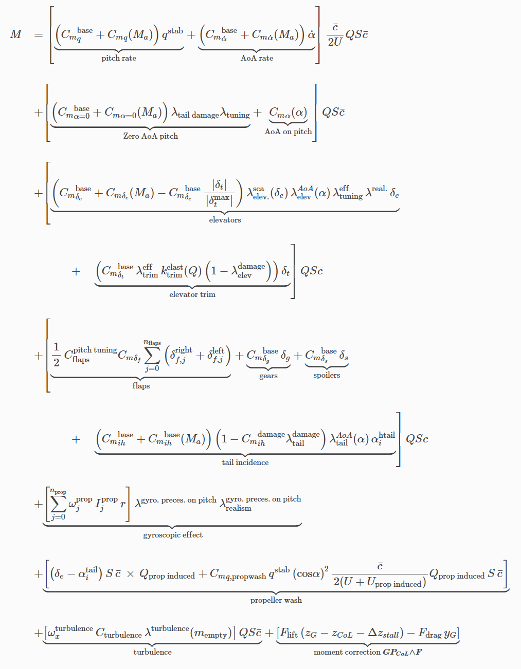
Finally, the yaw moment is computed as follows:

$$
\begin{array}{ll}
N &\displaystyle =
\left[
\underbrace{
\left({C_n}^{\textrm{base}}_r + {C_n}_r(M_a)\right)\,r^{\textrm{stab}}
}_{\textrm{yaw damping}}
+
\underbrace{
\left(
{C_n}^{\textrm{base}}_p + {C_n}_r(M_a)
\right)
\,\lambda^{\textrm{cross der. washout}}_{yaw}\left(\frac{\alpha}{\alpha^{\textrm{stall}}}\right)
\,p^{\textrm{stab}}
}_{\textrm{roll}}
\right]\,\frac{b}{2U}QSb
\\\\
&\displaystyle +
\left[
\underbrace{
{C_n}_{\alpha}(\alpha^{\textrm{lag}})\lambda^{\textrm{spin bias dir}}\lambda_{\textrm{realism}}
}_{\textrm{AoA}}
+
\underbrace{
\left({C_n}^{\textrm{base}}_{\beta} + {C_n}_{\beta}(M_a) \right)\,\lambda_{{C_n}_{\beta}}(\alpha)\,\left(1-\lambda^{\textrm{damage}}_{{C_n}_{\beta}}\right)
}_{\textrm{side slip}}
\right.
\\\\
&\displaystyle +
\left.
\underbrace{
\left({C_n}^{\textrm{base}}_{\delta r} + {C_n}_{\delta r}(M_a)\right)\,\lambda_{{C_n}_{\delta_r}}(\alpha)\,\lambda^{\textrm{scaling}}_{{C_n}_{\delta_r}}(\delta_r)
}_{\textrm{rudder}}
+
\underbrace{
{C_n}^{\textrm{base}}_{\delta r t} \delta_{rt}
}_{\textrm{rudder trim}}
\right.
\\\\
&\displaystyle \left.
+
\underbrace{
{C_n}^{\textrm{base, prop wash}}_{\delta r}\,\left(
\delta_r S b Q_{\textrm{prop induced}} b
+ r^{\textrm{stab}}\left(\textrm{cos}\alpha\right)^2
\frac{\bar{c}}{2U_{\textrm{prop induced}}} Q_{\textrm{prop induced}} S b
\right)
}_{\textrm{propeller wash on rudder}}
\right.
\\\\
&\displaystyle +
\left.
+
\underbrace{
\left(
{C_n}^{\textrm{base}}_{\delta a} + {C_n}_{\delta a}(M_a)
\right)\,\textrm{cos}\,\alpha
}_{\textrm{ailerons}}
\right.
\\\\
&\displaystyle
\left.
+ \underbrace
{
\frac{1}{2}\,{C_D}_{\delta_f}\lambda_{\textrm{tuning}}^{\textrm{flaps}}\,\sum_{j=0}^{n_{\textrm{flaps}}}\left(\delta_{f,j}^{\textrm{right}}-\delta_{f,j}^{\textrm{left}}\right)\,\frac{1}{2}\,c_{f}\, b
}_{\textrm{flaps}}
+ \underbrace{
F_{\textrm{drag}}\,\left(x_G - x_{\textrm{CoL}}\right) - F_{\textrm{side}}\,\left(z_G-z_{\textrm{CoL}}-\Delta z^{\textrm{stall}}\right)
}_{\textrm{moment correction } \boldsymbol{GP_{CoL}\wedge \boldsymbol{F}}}
\right]\,Q \,S\,b
\\\\
&\displaystyle
+ \textrm{gyroscopic effect on yaw}
+ \textrm{Pfactor moment}
+ \textrm{External Tank moment}\\\\
\end{array}$$

 

Potential flow theory $ = $ linked to rotational flow hypothesis \(\boldsymbol{\boldsymbol{U}} = 0\) In this case, if the fluid is in-compressible, potential \(\Phi\) is harmonic, i.e solution of \(\Delta \phi = 0\). A conformal mapping is a mapping that preserves angles and orientations locally. Generally, it is a complex function. Conformal mappings preserve harmonic functions, i.e: fields which are harmonic in the source domain are also harmonic in the image domain. This is useful for physical problems to get harmonic solutions around complex geometry by knowing harmonic solutions around simple geometry and transpose them around more complex geometries through conformal mapping. Joukowski theory uses this conformal mapping:

$$\boldsymbol{z} \rightarrow \boldsymbol{z}+ \frac{1}{\boldsymbol{z}}$$

 

To transform cylinders into airfoil profiles (with cusp trailing edge), the potential flow (i.e harmonic) solution around a cylinder is analytical and well known:

$$\left\{
\begin{array}{ll}
V_r &\displaystyle = U_{\infty}\left(1-\frac{R^2}{r^2}\right)\textrm{cos}\theta\\
V_{\theta} &\displaystyle = -U_{\infty}\left(1+\frac{R^2}{r^2}\right)\textrm{sin}\theta\\
p&\displaystyle =\frac{1}{2}\rho U_{\infty}^2 \left(2 \frac{R^2}{r^2} \textrm{cos}\left(2\theta\right) - \frac{R^4}{r^4}\right) +p_{\infty}
\end{array}
\right.$$

 

The solution of flow around a cylinder tells us that we should expect to find two stagnation points along the airfoil the position of which is determined by the circulation around the profile. There is a particular value of the circulation that moves the rear stagnation point (V=0) exactly on the trailing edge. This condition, which fixes a value of the circulation by simple geometrical considerations is the Kutta condition:

 

The Kutta conditions aims to reintroduce some "viscous" physics by selecting one specific "physical" solution among all potential flow complex solutions given by the Joulowski theory.

 

The theorem applies to two-dimensional flow around a fixed airfoil (or any shape of infinite span). The lift per unit span \(L\) of the airfoil is given by:

$$L'(x) = - \rho_{\infty}U_{\infty} \Gamma(x)$$

 

Where \(\rho_{\infty}\) and \(U_{\infty}\) are the fluid density and the fluid velocity far upstream of the airfoil, and \(\Gamma(x)\) is the circulation defined as the line integral:

$$\Gamma(x) = \int_{\mathcal{C}}{\boldsymbol{u}(\boldsymbol{s})\cdot\mathrm{d}\boldsymbol{s}}$$

 

Around a closed contour \(\mathcal{C}\) enclosing the airfoil and followed in the positive (anti-clockwise) direction. As explained below, this path must be in a region of potential flow and not in the boundary layer of the cylinder.

 

For a heuristic argument, consider a thin airfoil of chord \(c\) and infinite span, moving through air of density \(\rho\). Let the airfoil be inclined to the oncoming flow to produce an air speed \(U\) on one side of the airfoil, and an air speed \(U+v\) on the other side. The circulation is then:

$$\Gamma = U c - (U+v)c$$

 

The difference in pressure \(\) between the two sides of the airfoil is given by Bernouilli equations:

$$\begin{array}{ll}
&\frac{\rho}{2}U^2+(p+\Delta p) = \frac{\rho}{2}(U+v)^2+p\\
\Rightarrow &\frac{\rho}{2}U^2 + \Delta p = \frac{\rho}{2}(U^2 +2Uv + v^2)\\
\Rightarrow & \Delta p \approx \rho U v
\end{array}$$

 

So the lift per unit span is:

$$L'(x) = c(x)\Delta p = \rho Uvc= -\rho U \Gamma(x)$$

 

 

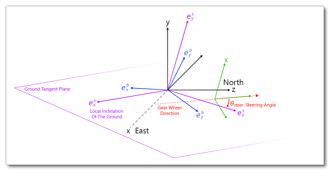
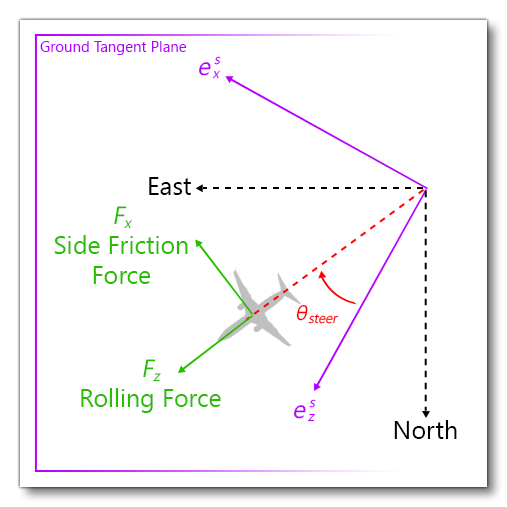
Contact Gear Forces

The images below are related to the forces acting on an aircraft when on the ground and the gear is out:

$$\boldsymbol{F}_{\textrm{ground reaction}}^b(t) = \mathcal{R}^{\textrm{surf} \rightarrow \textrm{body}}(t)\, \boldsymbol{F}_{\textrm{ground reaction}}^s(t)
= \left(\mathcal{R}^{\textrm{surf} \rightarrow \textrm{body}}\right)^{-1}(t)\, \boldsymbol{F}_{\textrm{ground reaction}}^s(t)$$

 

The strut force is a "penalization" reaction force, proportional to the vertical penetration of the gear in the ground:

$$F_{\textrm{strut}} = K_{\textrm{spring}}\, \underbrace{\textrm{min}\left(\textrm{max}\left(0,\, -y_{\textrm{agl}}\right),\, C_{\textrm{max compression}}\right)}_{\textrm{compression}} - K_{\textrm{damping}}\, v_y$$

 

This strut force represents the vertical reaction of the ground due to penetration in the aircraft body frame, i.e colinear to aircraft frame vertical direction \(\boldsymbol{e}^b_y\). Using the surface transformation matrix from body to surface frame as expressed above, we get:

$$\begin{array}{ll}
& \displaystyle \underbrace{F_y^b}_{\textrm{estimated strut force}} = r_{inv, 20} F_z^s + r_{inv, 21} F_x^s + r_{inv, 22} F_y^s\\\\
\Rightarrow & \displaystyle F_y^s = \frac{1}{r_{inv, 22}} \left(F_{strut} - r_{inv, 20} F_z^s - r_{inv, 21} F_x^s\right)
\end{array}$$

 

Regarding the integration scheme, as \(F_x^s\) and \(F_z^s\) are not know at \(t^n\), their value at \(t^{n-1}\) is used to evaluate \(F_y^s\):

$$F_y^{s, n} = \frac{1}{r_{inv, 22}} \left(F_{strut, n} - r_{inv, 20} F_z^{s, n-1} - r_{inv, 21} F_x^{s, n-1}\right)$$

 

The rolling friction force amplitude is computed as follows:

$$F_{\textrm{rolling friction}} = \left(C_{\textrm{rolling resistance}} + C_{\textrm{braking resistance}}\right) \times F_y^s$$

 

To compute side friction, we must first define these notions:

• Gear velocity
• Steering angle
• Slip angle

 

The gear velocity in body coordinates is easily computed from the gear position \(P_{gear}\) provided by the user in the reference datum frame and the current computed state of the aircraft:

$$\boldsymbol{v}^b_{\textrm{wheel}} = \boldsymbol{v}^b_G + \boldsymbol{\omega}^b\wedge \boldsymbol{G P_{\textrm{gear}}}^b$$

 

The steering angle requires a little more work. In the plane \(\left(\boldsymbol{e}^s_x, \boldsymbol{e}^s_z\right)\) locally tangent to the earth surface, the steering angle is the angle between the longitudinal axis of the wheel and the longitudinal direction of the aircraft projected on the plane \(\boldsymbol{e}^s_z\) (surface frame has been designed such that surface frame and aircraft body frame have the same yaw/heading). It is defined according to the user joystick/control input:

$$\theta_{\textrm{steer}} = C_{\textrm{max steering angle}} \times \lambda_{\textrm{steer input}} \times \lambda_{corr}\left(v_{\textrm{wheel}}\right)$$

 

Where \(\lambda_{\textrm{steer input}}\) is the scaling factor linked to current user seering input and \(\lambda_{corr}\) is a correction scaling to avoid over-controlling at faster speeds:

$$\lambda_{corr} = \lambda_{corr}\left(v_{\textrm{wheel}}\right) = \left\{
\begin{array}{ll}
1 & \textrm{if } v_{\textrm{wheel}} < v_{\textrm{min}}\\
1 + (\lambda_{corr, max} -1)\,\frac{v_{\textrm{wheel}}-v_{\textrm{min}}}{v_{\textrm{max}}-v_{\textrm{min}}} & \textrm{if } v_{\textrm{min}} < v_{\textrm{wheel}} < v_{\textrm{max}}\\
\lambda_{corr, max}& \textrm{if } v_{\textrm{wheel}} > v_{\textrm{max}}\\
\end{array}
\right.$$

With \(v_{\textrm{max}} = 50 \,\textrm{fps}\), \(v_{\textrm{min}} = 20 \,\textrm{fps}\), \(\lambda_{corr, max} = 0.25\).

 

Finally, the slip angle is the angle between the wheel longitudinal direction and the aircraft velocity direction:

$$\theta_{\textrm{slip}} = \theta_{\textrm{steer}} - \textrm{atan}\left(\frac{v_x^b}{v_z^b}\right)$$

 

The side friction force amplitude is computed as follows:

$$F_{\textrm{side friction}} = C_{\textrm{side friction}} \times \lambda(\theta_{\textrm{slip}})\times F_y^s$$

 

Where \(\lambda = \lambda(\theta_{\textrm{steer}})\) is a table that enables to weighten the friction depending on the slip angle. If the wheel is orthogonal to the longitudinal direction of the plane, friction is maximal and this coefficient is set to 1. On the contrary, if the wheel is perfectly aligned with the plane advancement direction, it is set to 0 and side friction is null.

 

Several empirical/experimental tables are set in hard in the code to provide friction and braking coefficients \(C_{\textrm{side friction}}\), \(C_{\textrm{rolling resistance}}\) and \(C_{\textrm{braking resistance}}\) depending on:

• the type of contact (eg: wheels, skids, scrape points, etc...)
• the type of surface (eg: concrete, snow, grass, etc...)
• the surface condition (eg: normal, wet, icy, etc...)

 

Ground Friction

Ground friction is simulated for aircraft within Microsoft Flight Simulator but is not currently available to be edited. It is based on a series of coefficient tables, from which we can extract the following information:

Friction	Tarmac	Low Speed Coefficient	High Speed Coefficient
Tire static friction	Dry	1.0	0.9
Tire dynamic friction	Dry	0.8	0.7
Tire static friction	Wet	0.6	0.54
Tire dynamic friction	Wet	0.6	0.54

 

All coefficients are expressed as in the coulomb model:

$$F_f \leq \mu F_n$$

where

• \(F_f\) is the force of friction exerted by each surface on the other. It is parallel to the surface, in a direction opposite to the net applied force.
• \(\mu\) is the coefficient of friction, which is an empirical property of the contacting materials,
• \(F_n\) is the normal force exerted by each surface on the other, directed perpendicular (normal) to the surface.

Using this model it is important to note that weight does not play a significant role on tarmac and only the friction coefficients do.

 

It is worth noting that

• braking force can never exceed tire/tarmac static friction otherwise it would make the tire skid and switch over to dynamic friction
• the toe braking coefficient defines braking resistance that has to be below tire static friction or the tire will skid. Usually we tend to set it at a lower coefficient so that we don’t risk skidding, even on wet surfaces.
• at very low speed, braking power is scaled up by 220% (always limited by static friction), in order to hold the plane in place when stopped.

 

Currently surfaces other than tarmac are not simulated in terms of friction. However, most other surfaces are considerably more bumpy, which in turn will automatically affect friction and braking distances just as in real life.

 

 

Ram Drag

Ram drag is the drag generated by the air that a turbine engine ingests to produce thrust. Essentially, all the air entering the engine inlet generates drag and that drag is calculated through the following formula:

$$D_{ram}=\frac{dm_0}{dt} \times V_0$$

Where:

• \(\frac{dm_0}{dt}\) is the mass flow (kg/s or lb/s).
• \(V_0\) is the speed of the incoming airflow (or mass flow). Note that "airflow" is an interpolation of the parameter corrected_airflow_table multiplied by the parameter inlet_area, both of which can be set in engines.cfg.

Because we need to be able to tune this ram drag effect we are simulating this formula like this:

$$D_{ram} = a(\rho,P) \times Ma_{inlet} \times airflow/g$$

Where:

• \(a(\rho,P)\) is the speed of sound in the current flight conditions
• \(Ma_{inlet}\) is the inlet Mach number
• \(airflow\) is a term dependent on the inlet design and computed through interpolation and correction using a cfg table and \(g\) the gravity constant of Earth.
• the product \(a \times Ma_{inlet}\) gives the previously stated \(V_0\).

 

The inlet simulation acts on \(Ma_{inlet}\) by either limiting it to 0.5 - if variable_inlet = 1 - or limiting it to 1.0 - if variable_inlet = 0 - as set in the engines.cfg file.

 

By default the simulation will compute the ram drag for a turbine engine using a maximum mach value of 1. However if you wish to add supersonic (even hypersonic) planes to the simulator then this will have the consequence of creating an inferior airflow speed leading to less drag than there should be. To correct this issue, the parameter supersonic_ram_drag should be set to 1 (true) in the [TURBINEENGINEDATA] section of the CFG file for the aircraft. Setting it to 1 will allow for the simulation to use the flight Mach number instead of the inlet Mach number thus removing the default Mach 1 limit.

 

 

Turbine Engine Supersonic Inlet

By default, the pressure increase on a turbine engine due to an increase in mach number (or total pressure recovery) is calculated using the inlet mach number which normally cannot exceed 1. This means that an aircraft which is supposed to fly faster than mach 1.0 at high altitudes will lose power due to the altitude (altitude pressure loss) but have minimal power gain from flying fast.

 

Total pressure recovery is the ability of an inlet to "recover" some of the total pressure of the ambient airstream, which increases with the flight mach number \(Ma\), thus allowing the inlet to have higher total pressure at the compressor face leading to an increase in power from the engine.

The default pressure recovery calculations are:

$$Pt_0 = P \times \frac{(Pt_0)}{P}$$

$$Pt_2 = Pt_0$$

Where:

• \(Pt_2\) is the total pressure at the compressor face
• \(P\) is the ambient pressure
• \(Pt_0\) the total pressure of the incoming airstream

This formula implies that the pressure recovery is done with an efficiency of 1. Also note that the default inlet simulation limits \(Ma_{inlet}\) to a maximum of 1.0, so the ratio \(\frac{(Pt_0)}{P}\) will not increase when \(Ma\) goes over 1.0. That means that an aircraft flying at Mach 1.6 will not benefit from a better pressure recovery.

 

This can be resolved using the supersonic inlet feature, which - when activated - allows for total pressure recovery to be calculated using a mach number above 1 and also allows for high-speed high altitude engine operation. This feature is enabled using the supersonic_inlet parameter in the [TURBINEENGINEDATA] section of the engines.cfg file.

 

When activated the inlet conditions calculations are divided between subsonic, supersonic and hypersonic conditions (only when the parameter supersonic_inlet_hypersonic is set to 1), and we determine \(η(Ma)\) from the supersonic_inlet_efficiency_correction_table table. Then the ratios \(\frac{Tt_0}{T}\) and \(\frac{Pt_0}{P}\) are computed using the flight mach number, \(Ma\), which means no limitations on these ratios. From these we can compute \(Pt_0\) and \(Tt_0\). \(Ma_{inlet}\) is then reduced to the value of supersonic_inlet_design_mach and \(Tt_2\) is calculated with this mach number.

 

The common assumption is to assume that compression is adiabatic therefore \(Tt_2 = Tt_0\). However due to the different corrections that happen in the simulation of the engine, this would lead to huge temperature and RPM increases and a drastic fuel flow decrease. This means that this part is not 100% realistic but has been necessary to avoid unrealistic results.

 

\(Pt_2\) is computed using the following rules and formulas:

$$Pt_2 = \eta(Ma) \times Pt_0 \text{ when } Ma<1 \text{ (subsonic conditions)}$$

$$Pt_2 = \eta(Ma) \times (1 - 0.075 \times (Ma - 1)^{1.35} ) \times Pt_0 \text{ when } Ma>1 \text{ (supersonic conditions)}$$

Note that the supersonic condition formulas will return a negative number when \(Ma\geq8\). To allow for hypersonic flight above mach 8 - an efficiency curve was established from a variety of academic papers on hypersonic inlet - giving the following calculation:

$$Pt_2 = \eta(Ma) \times \eta_{hypersonic} (Ma) \times Pt_0 \text{ when } Ma > 5$$

With \(\eta_{hypersonic}\) being a second order polynomial. In this situation the efficiency loss rate is equivalent to supersonic conditions, but at Mach 5.1 the resulting efficiency is 50% higher allowing for more pressure recovery. To use this efficiency increase when above Mach 5, the parameter supersonic_inlet_hypersonic must be set to 1, which will permit high-altitude, high-speed operation without the need of unrealistic amount of thrust at sea level.

 

 

Additional Information

This section contains additional information about the flight model that the simulation uses, in particular with reference to legacy products like Microsoft Flight Simulator X.

 

To start with, a new surface elements model has been created to better account for the distribution of lift, drag and side forces over the entire aircraft geometry. Compared to other flight simulators out there, our geometrical discretisation is more precise - our model uses 640 surfaces where other simulators have only ten elements per side per wing or stabilizer.

 

Our surface elements are spread out as follows:

• 40 x 3 for the fuselage, assimilated to an elongated rectangular box
• 1 x 3 for the gears, a box
• 1 x 3 for each external fuel tank, a box
• 20 x 3 for the vertical tail and rudder
• 20 x 3 for the horizontal tail and elevators
• 80 x 5 for each wing

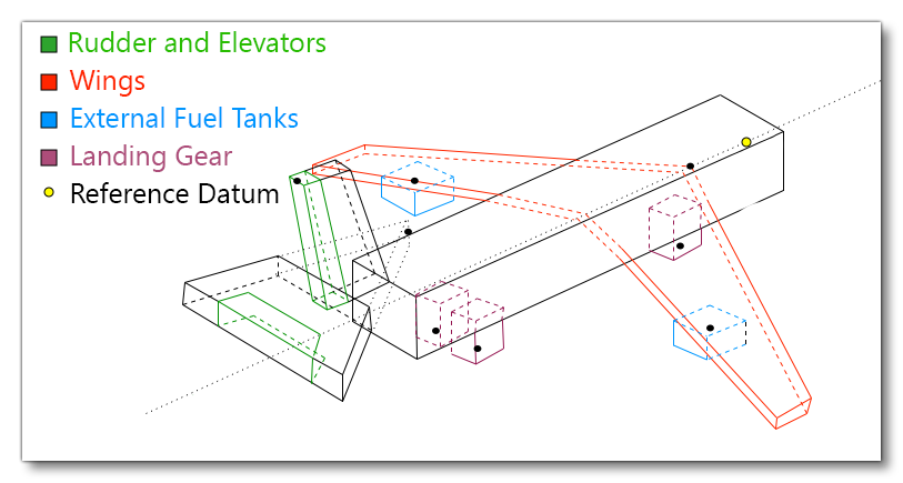
As depicted in the above figure, all geometrical elements of the aircraft are taken into account whereas in other simulators, only the wings, vertical stabilizer, horizontal stabilizer, and propellers are discretised. This means, for instance, that additional drag and pitch due to gears for cannot be accounted for in their model, while it can be in ours.

 

Normalization Algorithm

This algorithm is used to compute aerodynamics coefficients of each surface element. Indeed, we do not simulate the fluid movement around the aircraft at the moment so we must find a way to tell how each surface elements contribute to lift, drag, side forces and moments. One guideline we want to follow when attributing local aerodynamics coefficients to each surface is to ensure consistency with the classical aerodynamics theory underlying the legacy FSX flight model. To this end, an original normalization algorithm has been developed that helps redistribute global aerodynamics coefficients and tables - as provided by user - across all surface elements so that the final forces and moments match the ones computed by FSX. Of course, this does not mean we are finally equivalent to FSX modelling, as forces are now distributed over all the aircraft geometry. Instead it means that - when summing up all contributions and thus losing geometrical distribution information - our more general model can be reduced down to an approximation of the FSX legacy model. This makes our model an extension of the legacy model, which is in accordance with the objective of retro-compatibility. One great advantage of this is to guarantee a consistent behavior for aircraft designed with the legacy model when used in the new simulator under the improved flight model.

 

The normalization algorithm employed Microsoft Flight Simulator by is performed only once at the beginning of the game session. The idea behind it is to pre-compute during this initialization stage the following normalization coefficients:

• lift
• drag
• side
• moments

This will give a set of pre-defined control configurations. More precisely, 20 configurations involving flaps and spoiler deflections have been chosen. For each of these 20 aircraft control configurations, 6 normalization coefficients are computed and stored. A detailed explanation of how these normalization coefficients are computed is provided further down this page.

 

During the game, at each simulation step, this big look-up table linking a given control state to a set of normalization coefficients will be used to linearly interpolate current normalization coefficients from the current aircraft control configuration as input by the player. This interpolated set of normalization coefficients is then used to uniformly weight the lift and drag forces and the moments computed on each surface element, so that the simulation reaches the same global "zero order" solution as the one we would have computed with the FSX legacy model.

 

Now to explain how these normalization coefficients are computed for each of the 20 chosen aircraft control configurations during the initialization stage...

 

Let us consider a given controls configuration, with spoilers and flaps deflection angles set to a given value. We first use the FSX model to get the following eight values with the given flaps and spoilers deflection angles:

• \(C_L(\alpha =0)\)
• \(\mathrm{d}C_L = \frac{C_L(\alpha = 0.8\,\alpha_{\textrm{stall}}) - C_L(\alpha = 0)}{ (0.8\,\alpha_{\textrm{stall}})}\)
• \(C_m(\alpha =0)\)
• \(\mathrm{d}C_m = \frac{C_m(\alpha = 0.8\,\alpha_{\textrm{stall}}) -C_m(\alpha = 0)}{ (0.8\,\alpha_{\textrm{stall}})}\)
• \({C_m}_q\)
• \({C_n}_r\)
• \({C_l}_p\)
• \(\alpha = 0\)

 

We then initialize the algorithm by attributing - to each surface element - local lift, drag and moments coefficients, simply by uniformly distributing aerodynamics coefficients and tables provided by the user over all surface elements with a basic surface-area-based weighting. We then iteratively compute the same 8 global coefficients we have retrieved from FSX as explained above, but using the new surface elements model. To do so, the surface elements model is evaluated on 6 different aircraft states:

• Zero angle-of-attack (purely frontal relative wind) and aircraft has no rotation speed
• 10 degrees angle-of-attack and aircraft has no rotation speed
• Purely sided relative wind and aircraft has no rotation speed
• Zero angle of attack and aircraft has pure constant pitch velocity of 0.5 FPS
• Zero angle of attack and aircraft has pure constant roll velocity of 0.5 FPS
• Zero angle of attack and aircraft has pure constant yaw velocity of 0.5 FPS

 

These 6 states excite all modes of the surface element models and enables us to estimate the 8 global coefficients: \(C_L(\alpha =0)\), \(\mathrm{d}C_L\)m, \(C_D(\alpha =0)\), \(C_m(\alpha =0)\), \(\mathrm{d}C_m\) and stability derivatives. At the end of each iteration, we correct the surface elements local aerodynamics coefficients - uniformly multiplying surface elements lift, drag, side, and moments coefficients by a ratio comparing FSX legacy models with the new model. With this we can a-posteriori reach the FSX global target. This evaluation/correction is performed until no correction is needed, i.e: the correction ratio stagnates to 1. At the end of this iterative loop, we have attributed lift/drag/side and moments coefficients to each surface element and we can guarantee that the contributions of all surface elements, when summed up, lead to the same "zero order" solution as the one previously obtained in FSX.

 

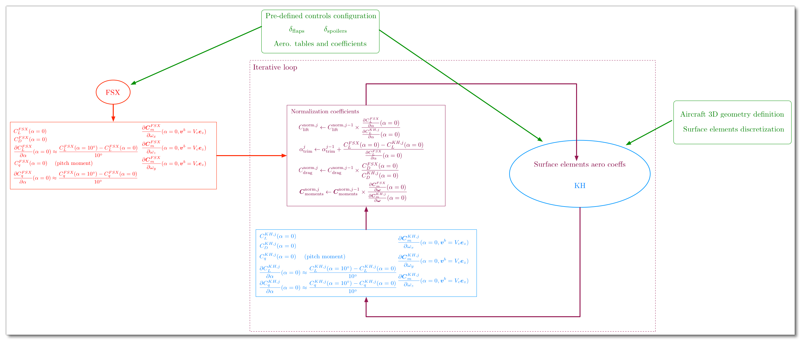
Stall Modelisation

When an aircraft is flying normally, the air moves across the wing in a smooth stream. If the aircraft is pitched upwards sufficiently, the air stream becomes less fluid until it finally "detaches" from the wing. This is called a "stall". Microsoft Flight Simulator X had a stall model, but the stalls weren't entirely native to the simulation. That is, when the conditions for a stall occurred, some additional code would take over to simulate the stall, as a global phenomenon. While using the FSX legacy flight model, experienced pilots collaborating with us have noticed poor behavior for limit cases - typically when approaching stall - which has motivated the team behind Microsoft Flight Simulator to put some additional effort into physical modelling of limit flight configurations, which are notoriously badly represented in the classical aerodynamics theory underlying the FSX legacy flight model.

 

The introduction of 3D geometrical information in the flight model through surface elements, as described in the previous section, was clearly a first mandatory step toward improving the physics, as it has enabled the modelisation of local phenomena. To better account for stall and all its variants (spin stall, deep stall, simple stall), each surface element has been enriched with a float parameter describing its level of stall. When reaching a certain level of stall, the behavior of the surface is changed using additional parameters so as to follow, broadly speaking, the behavior of a "falling plate" (ie: the post-stall aerodynamic characteristics of a generic 2D airfoil, which can be likened to a flat plate). If you'd like further information you can read the following articles:

• Airfoils at High Angle of Attack
• Airfoil Section At Angles Of Attack From 0 Degrees To 180 Degrees

 

This "plate" model is used in the new flight model to locally change the behavior of surface elements depending on local stall state. This enables us to accurately simulate classical stall but also spin stall, which is intrinsically impossible with the FSX non-geometrical flight model. The effect of geometrically twisted wings on stall, which tends to delay stall as the wing root stalls before the wing tip, is also clearly simulated and can even be depicted in-game using debug mode. In the same way, a spin stall is like a normal stall, but it happens to only one wing of the aircraft. When one wing has lift and the other does not, the flying wing will continue to rise until it flips the plane. Without geometrical input in the flight model, the legacy FSX model could not really account for spin stall, which is now the case with the new flight model.

 

 

Interferences And Geometrical Self-perturbation Modelisation

We also believe that our new flight model has some notable and measurable advantages over other flight simulators due to surface inter-dependency: a surface hit by air will create a change in the airflow that will impact all other surfaces behind the first surface, an effect which is essential for simulating (among other things):

• Engine wash
• Shadowing
• Deep stall

 

Geometrical analysis with respect to the flow direction is performed in the simulation code. This enables us to spot which surface elements are shadowed or washed and to temporarily alter their lifting properties accordingly. Future work using the 3D visual model will help improve the computation of occluded/washed surfaces - for instance using ray tracing.